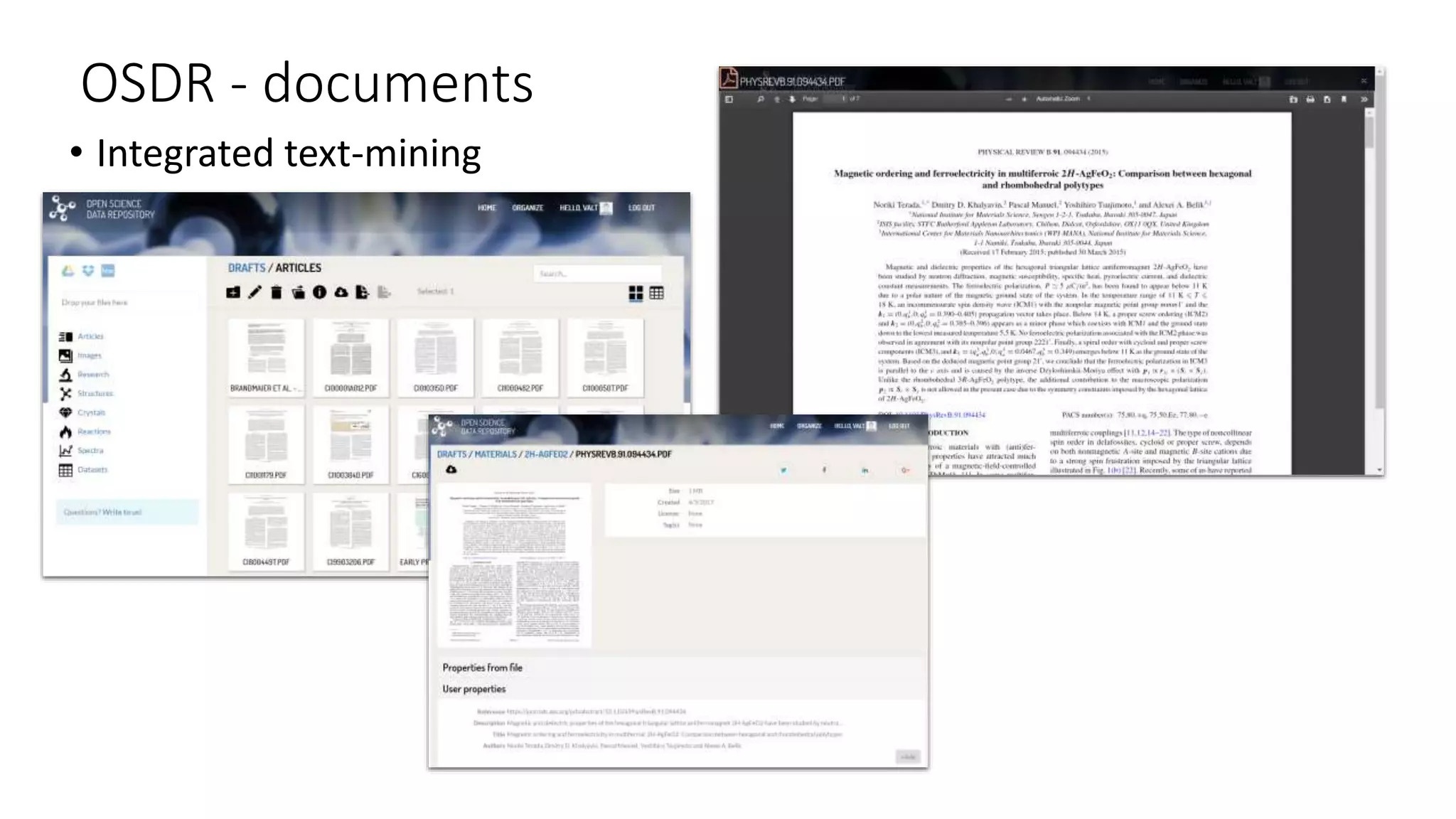
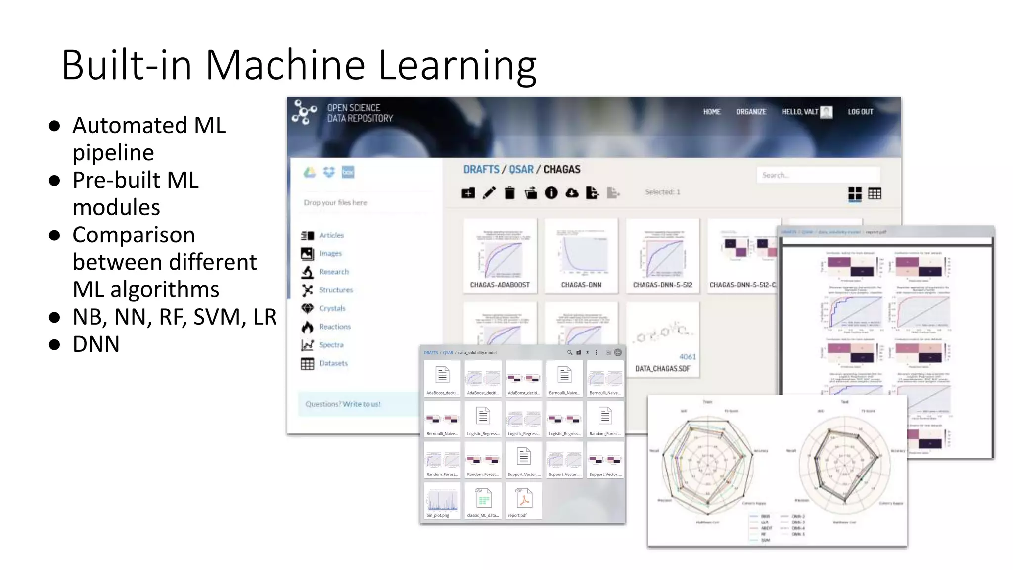
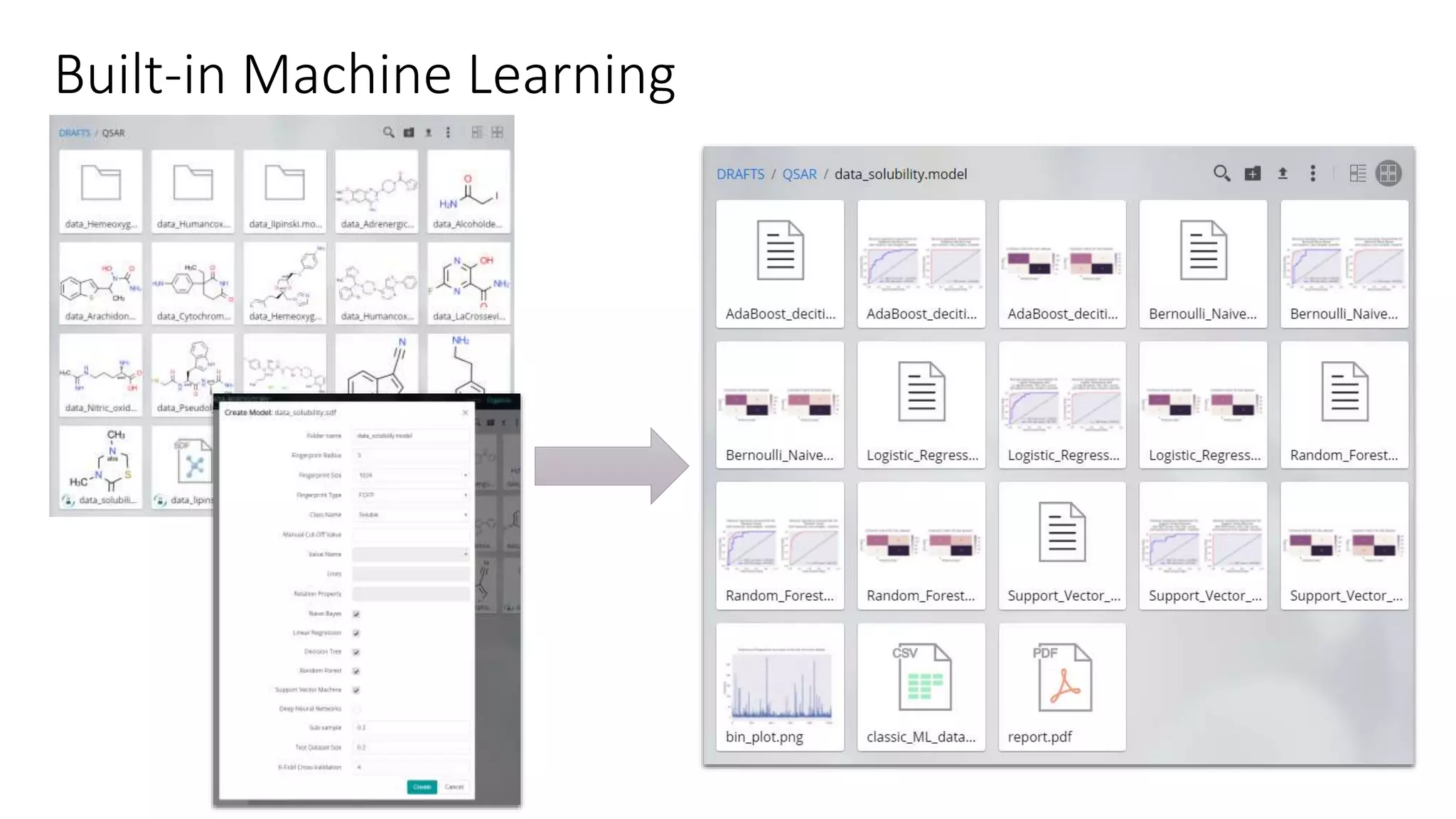
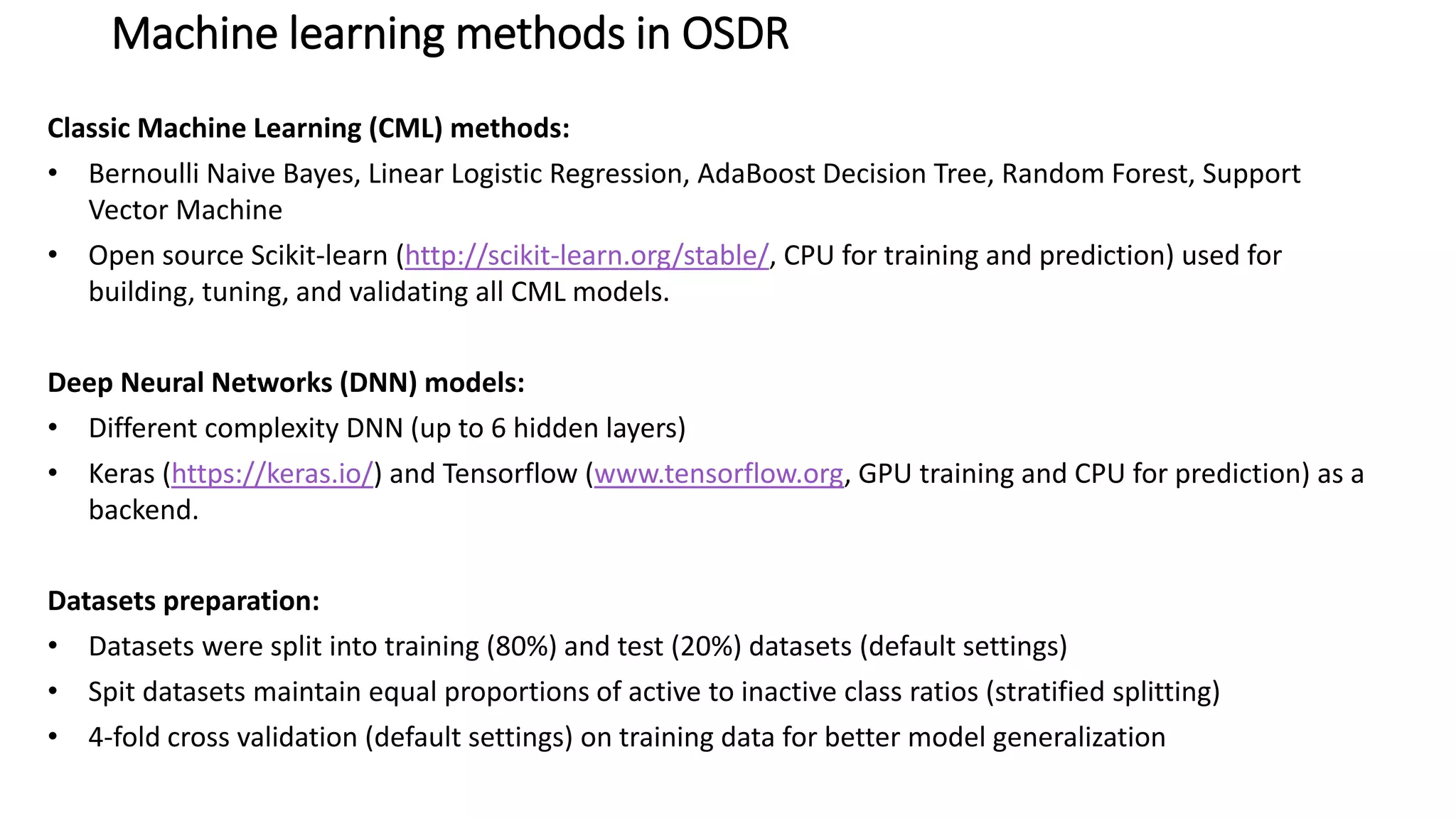
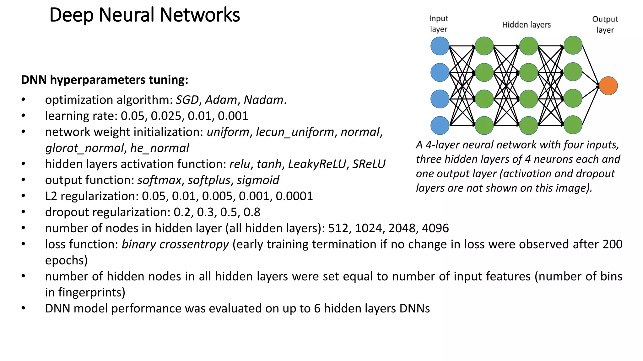
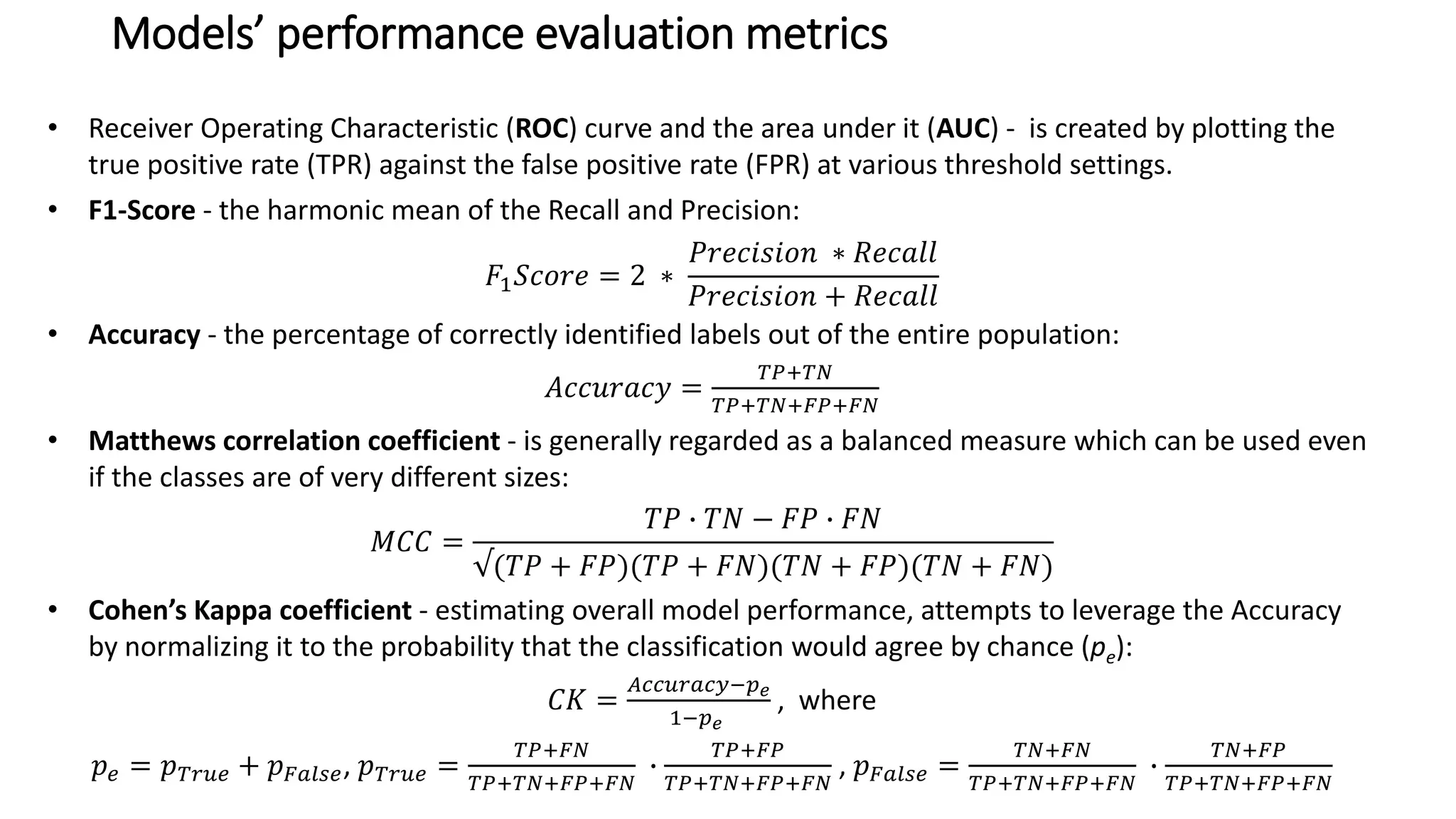
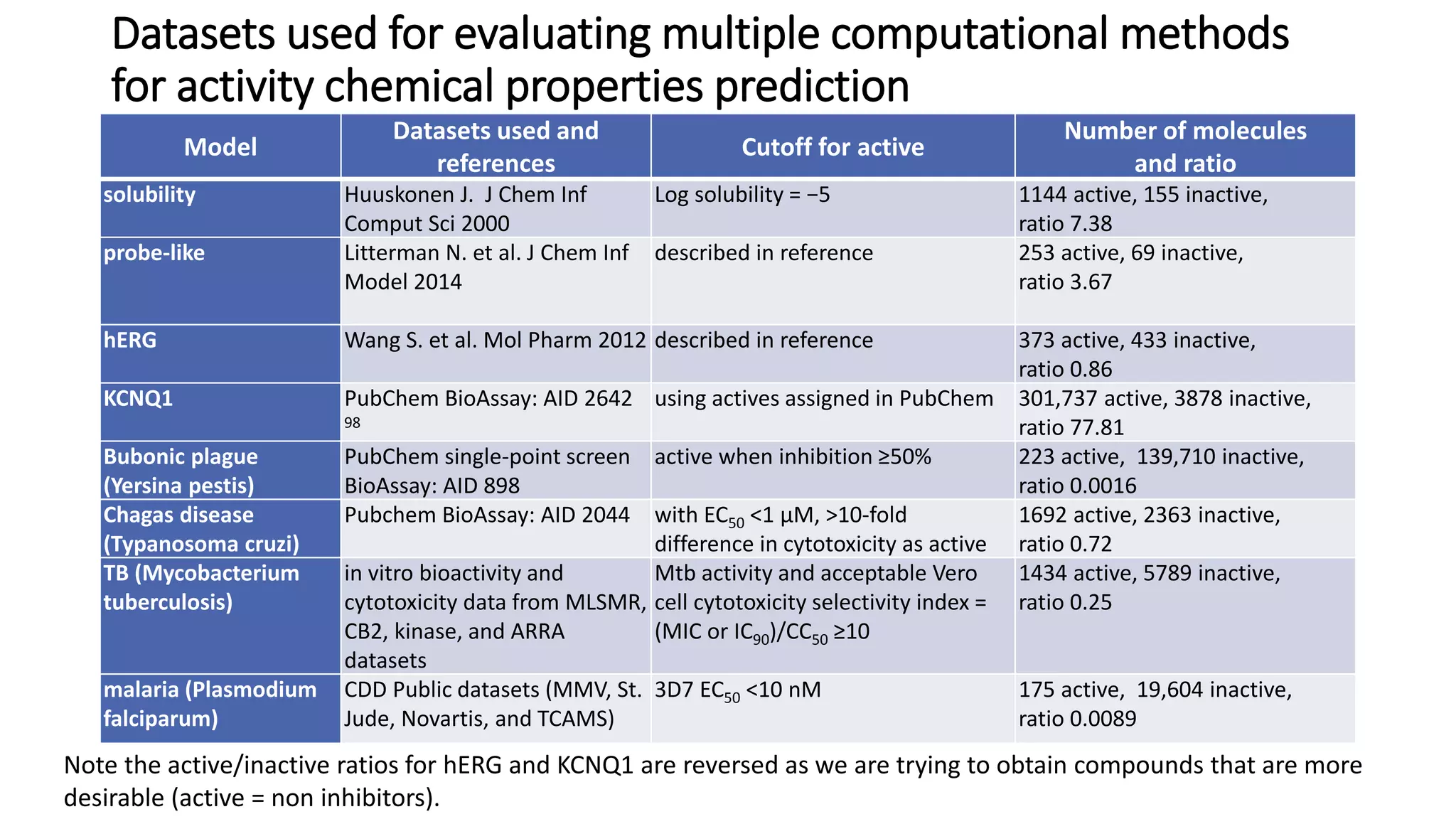
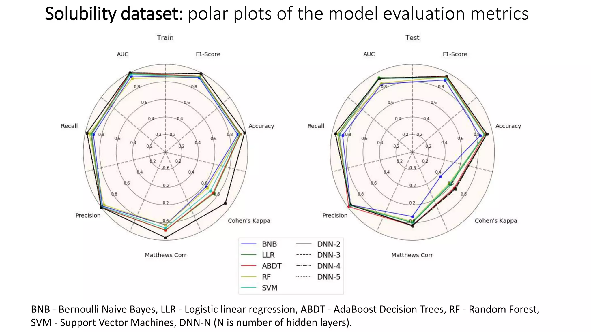
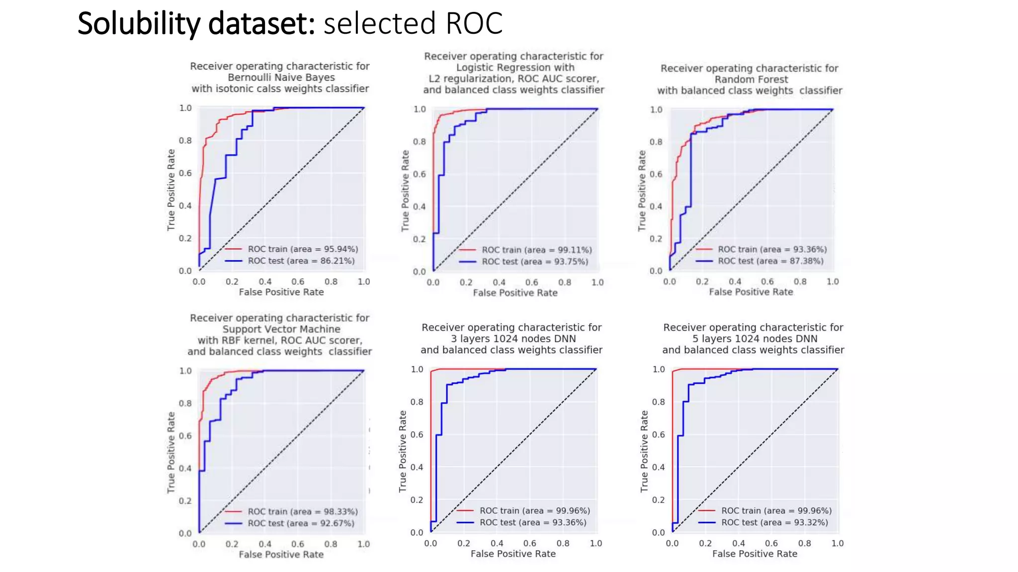
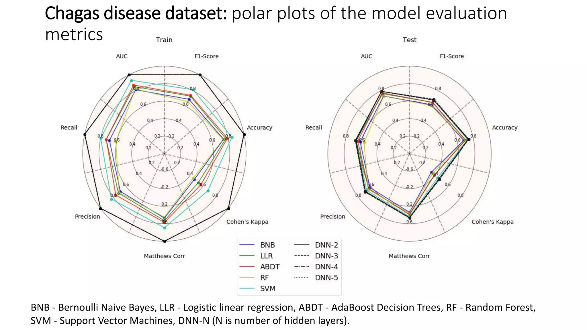
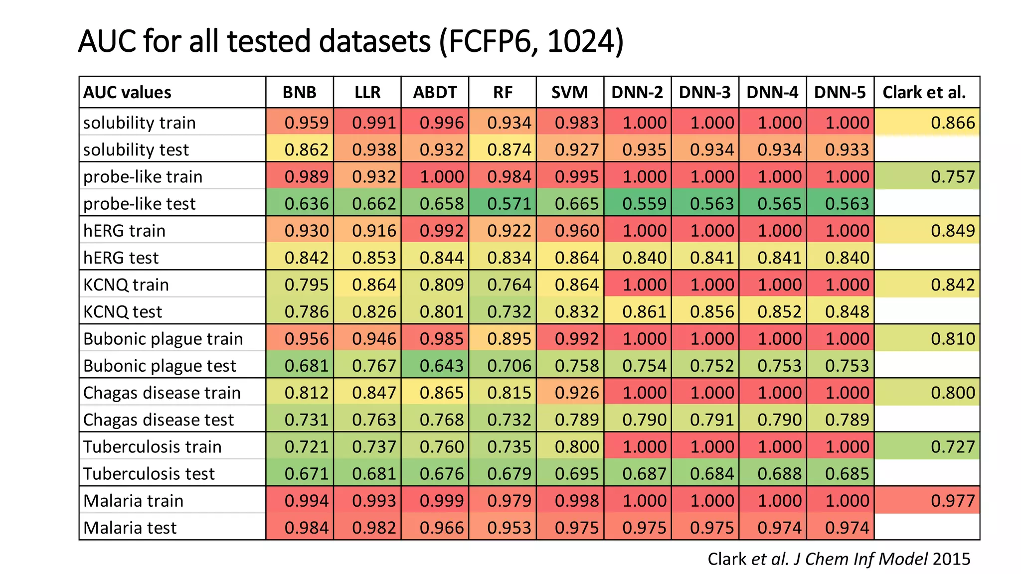
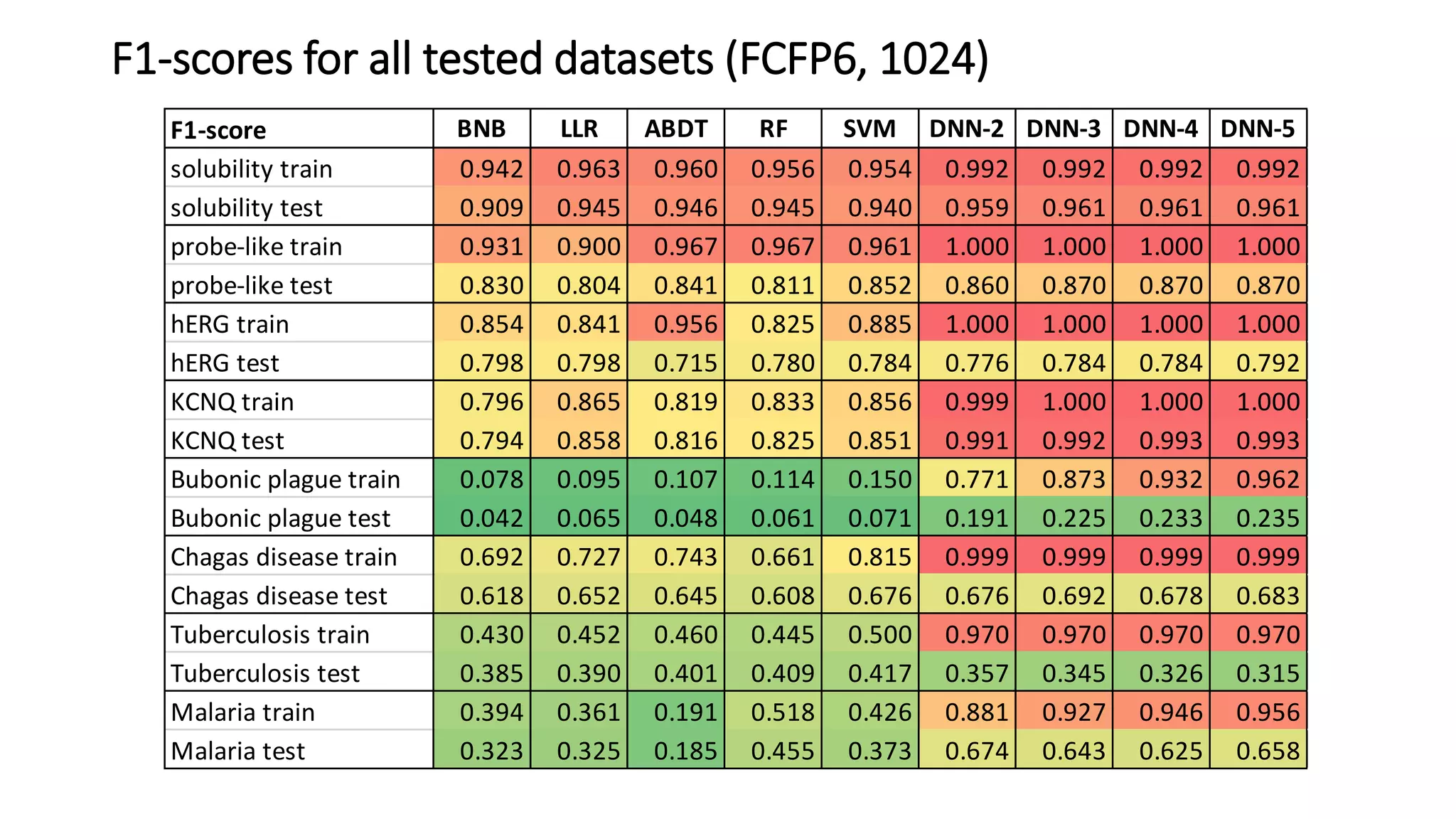
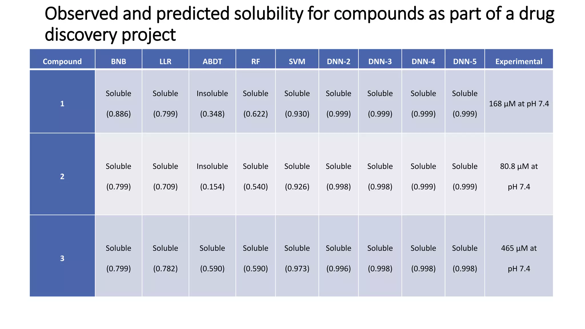
Development and comparison
of deep learning toolkit with
other machine learning
methods
Valery Tkachenko2, Boris Sattarov2, Artem Mitrofanov3, Alexandru Korotcov2,
Sean Ekins1
1Collaborations Pharmaceuticals, Fuquay Varina, North Carolina, United States
2SCIENCE DATA SOFTWARE, LLC, Rockville, Maryland, United States
3Chemistry Department, Moscow State University, Moscow, Russian Federation
D
a
t
a
Data Lake
Social
Media
Electronic
Notebooks
Databases
Sensor Med
Dev
IoT
Curated
Repository
Models
Curation &
Integration
Validation
Decision
Support
Analysis &
Modeling
Open Data Science Platform
Mining
USERS
Model-driven experimental studies
Extensible micro-service based architecture
Open Science Data Repository (OSDR)
Chemical processing
● Support for chemical
formats
● Chemistry validation
and standardization
● Automatic processing
and visualization
J. Brechner, IUPAC
Graphical Representation of
stereochem. configurations
Section: ST-1.1.10
DB06287
Chemical Lenses
OSDR - documents
• Integrated text-mining
FAIR Data Principles
Built-in Machine Learning
● Automated ML
pipeline
● Pre-built ML
modules
● Comparison
between different
ML algorithms
● NB, NN, RF, SVM, LR
● DNN
Built-in Machine Learning
In progress…
Machine learning methods in OSDR
Classic Machine Learning (CML) methods:
• Bernoulli Naive Bayes, Linear Logistic Regression, AdaBoost Decision Tree, Random Forest, Support
Vector Machine
• Open source Scikit-learn (http://scikit-learn.org/stable/, CPU for training and prediction) used for
building, tuning, and validating all CML models.
Deep Neural Networks (DNN) models:
• Different complexity DNN (up to 6 hidden layers)
• Keras (https://keras.io/) and Tensorflow (www.tensorflow.org, GPU training and CPU for prediction) as a
backend.
Datasets preparation:
• Datasets were split into training (80%) and test (20%) datasets (default settings)
• Spit datasets maintain equal proportions of active to inactive class ratios (stratified splitting)
• 4-fold cross validation (default settings) on training data for better model generalization
Deep Neural Networks
DNN hyperparameters tuning:
• optimization algorithm: SGD, Adam, Nadam.
• learning rate: 0.05, 0.025, 0.01, 0.001
• network weight initialization: uniform, lecun_uniform, normal,
glorot_normal, he_normal
• hidden layers activation function: relu, tanh, LeakyReLU, SReLU
• output function: softmax, softplus, sigmoid
• L2 regularization: 0.05, 0.01, 0.005, 0.001, 0.0001
• dropout regularization: 0.2, 0.3, 0.5, 0.8
• number of nodes in hidden layer (all hidden layers): 512, 1024, 2048, 4096
• loss function: binary crossentropy (early training termination if no change in loss were observed after 200
epochs)
• number of hidden nodes in all hidden layers were set equal to number of input features (number of bins
in fingerprints)
• DNN model performance was evaluated on up to 6 hidden layers DNNs
A 4-layer neural network with four inputs,
three hidden layers of 4 neurons each and
one output layer (activation and dropout
layers are not shown on this image).
Models’ performance evaluation metrics
• Receiver Operating Characteristic (ROC) curve and the area under it (AUC) - is created by plotting the
true positive rate (TPR) against the false positive rate (FPR) at various threshold settings.
• F1-Score - the harmonic mean of the Recall and Precision:
𝐹1 𝑆𝑐𝑜𝑟𝑒 = 2 ∗
𝑃𝑟𝑒𝑐𝑖𝑠𝑖𝑜𝑛 ∗ 𝑅𝑒𝑐𝑎𝑙𝑙
𝑃𝑟𝑒𝑐𝑖𝑠𝑖𝑜𝑛 + 𝑅𝑒𝑐𝑎𝑙𝑙
• Accuracy - the percentage of correctly identified labels out of the entire population:
𝐴𝑐𝑐𝑢𝑟𝑎𝑐𝑦 =
𝑇𝑃+𝑇𝑁
𝑇𝑃+𝑇𝑁+𝐹𝑃+𝐹𝑁
• Matthews correlation coefficient - is generally regarded as a balanced measure which can be used even
if the classes are of very different sizes:
𝑀𝐶𝐶 =
𝑇𝑃 ∙ 𝑇𝑁 − 𝐹𝑃 ∙ 𝐹𝑁
√(𝑇𝑃 + 𝐹𝑃)(𝑇𝑃 + 𝐹𝑁)(𝑇𝑁 + 𝐹𝑃)(𝑇𝑁 + 𝐹𝑁)
• Cohen’s Kappa coefficient - estimating overall model performance, attempts to leverage the Accuracy
by normalizing it to the probability that the classification would agree by chance (pe):
𝐶𝐾 =
𝐴𝑐𝑐𝑢𝑟𝑎𝑐𝑦−𝑝 𝑒
1−𝑝 𝑒
, where
𝑝 𝑒 = 𝑝 𝑇𝑟𝑢𝑒 + 𝑝 𝐹𝑎𝑙𝑠𝑒, 𝑝 𝑇𝑟𝑢𝑒 =
𝑇𝑃+𝐹𝑁
𝑇𝑃+𝑇𝑁+𝐹𝑃+𝐹𝑁
∙
𝑇𝑃+𝐹𝑃
𝑇𝑃+𝑇𝑁+𝐹𝑃+𝐹𝑁
, 𝑝 𝐹𝑎𝑙𝑠𝑒 =
𝑇𝑁+𝐹𝑁
𝑇𝑃+𝑇𝑁+𝐹𝑃+𝐹𝑁
∙
𝑇𝑁+𝐹𝑃
𝑇𝑃+𝑇𝑁+𝐹𝑃+𝐹𝑁
Datasets used for evaluating multiple computational methods
for activity chemical properties prediction
Model
Datasets used and
references
Cutoff for active
Number of molecules
and ratio
solubility Huuskonen J. J Chem Inf
Comput Sci 2000
Log solubility = −5 1144 active, 155 inactive,
ratio 7.38
probe-like Litterman N. et al. J Chem Inf
Model 2014
described in reference 253 active, 69 inactive,
ratio 3.67
hERG Wang S. et al. Mol Pharm 2012 described in reference 373 active, 433 inactive,
ratio 0.86
KCNQ1 PubChem BioAssay: AID 2642
98
using actives assigned in PubChem 301,737 active, 3878 inactive,
ratio 77.81
Bubonic plague
(Yersina pestis)
PubChem single-point screen
BioAssay: AID 898
active when inhibition ≥50% 223 active, 139,710 inactive,
ratio 0.0016
Chagas disease
(Typanosoma cruzi)
Pubchem BioAssay: AID 2044 with EC50 <1 μM, >10-fold
difference in cytotoxicity as active
1692 active, 2363 inactive,
ratio 0.72
TB (Mycobacterium
tuberculosis)
in vitro bioactivity and
cytotoxicity data from MLSMR,
CB2, kinase, and ARRA
datasets
Mtb activity and acceptable Vero
cell cytotoxicity selectivity index =
(MIC or IC90)/CC50 ≥10
1434 active, 5789 inactive,
ratio 0.25
malaria (Plasmodium
falciparum)
CDD Public datasets (MMV, St.
Jude, Novartis, and TCAMS)
3D7 EC50 <10 nM 175 active, 19,604 inactive,
ratio 0.0089
Note the active/inactive ratios for hERG and KCNQ1 are reversed as we are trying to obtain compounds that are more
desirable (active = non inhibitors).
Solubility dataset: polar plots of the model evaluation metrics
BNB - Bernoulli Naive Bayes, LLR - Logistic linear regression, ABDT - AdaBoost Decision Trees, RF - Random Forest,
SVM - Support Vector Machines, DNN-N (N is number of hidden layers).
Solubility dataset: selected ROC
BNB - Bernoulli Naive Bayes, LLR - Logistic linear regression, ABDT - AdaBoost Decision Trees, RF - Random Forest,
SVM - Support Vector Machines, DNN-N (N is number of hidden layers).
Chagas disease dataset: polar plots of the model evaluation
metrics
AUC for all tested datasets (FCFP6, 1024)
Clark et al. J Chem Inf Model 2015
AUC values BNB LLR ABDT RF SVM DNN-2 DNN-3 DNN-4 DNN-5 Clark et al.
solubility train 0.959 0.991 0.996 0.934 0.983 1.000 1.000 1.000 1.000 0.866
solubility test 0.862 0.938 0.932 0.874 0.927 0.935 0.934 0.934 0.933
probe-like train 0.989 0.932 1.000 0.984 0.995 1.000 1.000 1.000 1.000 0.757
probe-like test 0.636 0.662 0.658 0.571 0.665 0.559 0.563 0.565 0.563
hERG train 0.930 0.916 0.992 0.922 0.960 1.000 1.000 1.000 1.000 0.849
hERG test 0.842 0.853 0.844 0.834 0.864 0.840 0.841 0.841 0.840
KCNQ train 0.795 0.864 0.809 0.764 0.864 1.000 1.000 1.000 1.000 0.842
KCNQ test 0.786 0.826 0.801 0.732 0.832 0.861 0.856 0.852 0.848
Bubonic plague train 0.956 0.946 0.985 0.895 0.992 1.000 1.000 1.000 1.000 0.810
Bubonic plague test 0.681 0.767 0.643 0.706 0.758 0.754 0.752 0.753 0.753
Chagas disease train 0.812 0.847 0.865 0.815 0.926 1.000 1.000 1.000 1.000 0.800
Chagas disease test 0.731 0.763 0.768 0.732 0.789 0.790 0.791 0.790 0.789
Tuberculosis train 0.721 0.737 0.760 0.735 0.800 1.000 1.000 1.000 1.000 0.727
Tuberculosis test 0.671 0.681 0.676 0.679 0.695 0.687 0.684 0.688 0.685
Malaria train 0.994 0.993 0.999 0.979 0.998 1.000 1.000 1.000 1.000 0.977
Malaria test 0.984 0.982 0.966 0.953 0.975 0.975 0.975 0.974 0.974
F1-scores for all tested datasets (FCFP6, 1024)
F1-score BNB LLR ABDT RF SVM DNN-2 DNN-3 DNN-4 DNN-5
solubility train 0.942 0.963 0.960 0.956 0.954 0.992 0.992 0.992 0.992
solubility test 0.909 0.945 0.946 0.945 0.940 0.959 0.961 0.961 0.961
probe-like train 0.931 0.900 0.967 0.967 0.961 1.000 1.000 1.000 1.000
probe-like test 0.830 0.804 0.841 0.811 0.852 0.860 0.870 0.870 0.870
hERG train 0.854 0.841 0.956 0.825 0.885 1.000 1.000 1.000 1.000
hERG test 0.798 0.798 0.715 0.780 0.784 0.776 0.784 0.784 0.792
KCNQ train 0.796 0.865 0.819 0.833 0.856 0.999 1.000 1.000 1.000
KCNQ test 0.794 0.858 0.816 0.825 0.851 0.991 0.992 0.993 0.993
Bubonic plague train 0.078 0.095 0.107 0.114 0.150 0.771 0.873 0.932 0.962
Bubonic plague test 0.042 0.065 0.048 0.061 0.071 0.191 0.225 0.233 0.235
Chagas disease train 0.692 0.727 0.743 0.661 0.815 0.999 0.999 0.999 0.999
Chagas disease test 0.618 0.652 0.645 0.608 0.676 0.676 0.692 0.678 0.683
Tuberculosis train 0.430 0.452 0.460 0.445 0.500 0.970 0.970 0.970 0.970
Tuberculosis test 0.385 0.390 0.401 0.409 0.417 0.357 0.345 0.326 0.315
Malaria train 0.394 0.361 0.191 0.518 0.426 0.881 0.927 0.946 0.956
Malaria test 0.323 0.325 0.185 0.455 0.373 0.674 0.643 0.625 0.658
Observed and predicted solubility for compounds as part of a drug
discovery project
Compound BNB LLR ABDT RF SVM DNN-2 DNN-3 DNN-4 DNN-5 Experimental
1
Soluble
(0.886)
Soluble
(0.799)
Insoluble
(0.348)
Soluble
(0.622)
Soluble
(0.930)
Soluble
(0.999)
Soluble
(0.999)
Soluble
(0.999)
Soluble
(0.999)
168 µM at pH 7.4
2
Soluble
(0.799)
Soluble
(0.709)
Insoluble
(0.154)
Soluble
(0.540)
Soluble
(0.926)
Soluble
(0.998)
Soluble
(0.998)
Soluble
(0.999)
Soluble
(0.999)
80.8 µM at
pH 7.4
3
Soluble
(0.799)
Soluble
(0.782)
Soluble
(0.590)
Soluble
(0.590)
Soluble
(0.973)
Soluble
(0.996)
Soluble
(0.998)
Soluble
(0.998)
Soluble
(0.998)
465 µM at
pH 7.4
Summary
• A Machine Learning toolkit with simple user interface have been
developed for the Open Science Data Repository software.
• Two major pipelines are implemented: Classic Machine learning methods
(Bernoulli Naive Bayes, Linear Logistic Regression, AdaBoost Decision Tree,
Random Forest, Support Vector Machine), and Deep Neural Networks.
• Multiple models’ performance evaluation metrics, such as ROC, AUC, F1
score, Accuracy, Cohen’s kappa, and Matthews correlation coefficient
were implemented.
Summary
• All model were evaluated using relevant to pharmaceutical research
include absorption, distribution, metabolism, excretion and toxicity
(ADME/Tox) properties, as well as activity against pathogens and drug
discovery datasets.
• DNN learning models were found to be very good in predicting activities
and can outperform most of the CML models. The models were applied to
real world drug discovery task like assessing solubility, and exhibited very
good prediction performances.
• FCFP6 does quite well with the datasets in this study, but future studies
are needed to evaluate additional fingerprints such as or other non-
fingerprint descriptors with DNN.
Thank you!
On Web:
scidatasoft.com
Slides:
https://www.slideshare.net/valerytkachenko16
Contact us:
info@scidatasoft.com

Development and comparison of deep learning toolkit with other machine learning methods

  • 1.
    Development and comparison ofdeep learning toolkit with other machine learning methods Valery Tkachenko2, Boris Sattarov2, Artem Mitrofanov3, Alexandru Korotcov2, Sean Ekins1 1Collaborations Pharmaceuticals, Fuquay Varina, North Carolina, United States 2SCIENCE DATA SOFTWARE, LLC, Rockville, Maryland, United States 3Chemistry Department, Moscow State University, Moscow, Russian Federation
  • 3.
    D a t a Data Lake Social Media Electronic Notebooks Databases Sensor Med Dev IoT Curated Repository Models Curation& Integration Validation Decision Support Analysis & Modeling Open Data Science Platform Mining USERS Model-driven experimental studies
  • 4.
  • 5.
    Open Science DataRepository (OSDR)
  • 6.
    Chemical processing ● Supportfor chemical formats ● Chemistry validation and standardization ● Automatic processing and visualization
  • 8.
    J. Brechner, IUPAC GraphicalRepresentation of stereochem. configurations Section: ST-1.1.10 DB06287
  • 9.
  • 10.
    OSDR - documents •Integrated text-mining
  • 11.
  • 12.
    Built-in Machine Learning ●Automated ML pipeline ● Pre-built ML modules ● Comparison between different ML algorithms ● NB, NN, RF, SVM, LR ● DNN
  • 13.
  • 14.
  • 15.
    Machine learning methodsin OSDR Classic Machine Learning (CML) methods: • Bernoulli Naive Bayes, Linear Logistic Regression, AdaBoost Decision Tree, Random Forest, Support Vector Machine • Open source Scikit-learn (http://scikit-learn.org/stable/, CPU for training and prediction) used for building, tuning, and validating all CML models. Deep Neural Networks (DNN) models: • Different complexity DNN (up to 6 hidden layers) • Keras (https://keras.io/) and Tensorflow (www.tensorflow.org, GPU training and CPU for prediction) as a backend. Datasets preparation: • Datasets were split into training (80%) and test (20%) datasets (default settings) • Spit datasets maintain equal proportions of active to inactive class ratios (stratified splitting) • 4-fold cross validation (default settings) on training data for better model generalization
  • 16.
    Deep Neural Networks DNNhyperparameters tuning: • optimization algorithm: SGD, Adam, Nadam. • learning rate: 0.05, 0.025, 0.01, 0.001 • network weight initialization: uniform, lecun_uniform, normal, glorot_normal, he_normal • hidden layers activation function: relu, tanh, LeakyReLU, SReLU • output function: softmax, softplus, sigmoid • L2 regularization: 0.05, 0.01, 0.005, 0.001, 0.0001 • dropout regularization: 0.2, 0.3, 0.5, 0.8 • number of nodes in hidden layer (all hidden layers): 512, 1024, 2048, 4096 • loss function: binary crossentropy (early training termination if no change in loss were observed after 200 epochs) • number of hidden nodes in all hidden layers were set equal to number of input features (number of bins in fingerprints) • DNN model performance was evaluated on up to 6 hidden layers DNNs A 4-layer neural network with four inputs, three hidden layers of 4 neurons each and one output layer (activation and dropout layers are not shown on this image).
  • 17.
    Models’ performance evaluationmetrics • Receiver Operating Characteristic (ROC) curve and the area under it (AUC) - is created by plotting the true positive rate (TPR) against the false positive rate (FPR) at various threshold settings. • F1-Score - the harmonic mean of the Recall and Precision: 𝐹1 𝑆𝑐𝑜𝑟𝑒 = 2 ∗ 𝑃𝑟𝑒𝑐𝑖𝑠𝑖𝑜𝑛 ∗ 𝑅𝑒𝑐𝑎𝑙𝑙 𝑃𝑟𝑒𝑐𝑖𝑠𝑖𝑜𝑛 + 𝑅𝑒𝑐𝑎𝑙𝑙 • Accuracy - the percentage of correctly identified labels out of the entire population: 𝐴𝑐𝑐𝑢𝑟𝑎𝑐𝑦 = 𝑇𝑃+𝑇𝑁 𝑇𝑃+𝑇𝑁+𝐹𝑃+𝐹𝑁 • Matthews correlation coefficient - is generally regarded as a balanced measure which can be used even if the classes are of very different sizes: 𝑀𝐶𝐶 = 𝑇𝑃 ∙ 𝑇𝑁 − 𝐹𝑃 ∙ 𝐹𝑁 √(𝑇𝑃 + 𝐹𝑃)(𝑇𝑃 + 𝐹𝑁)(𝑇𝑁 + 𝐹𝑃)(𝑇𝑁 + 𝐹𝑁) • Cohen’s Kappa coefficient - estimating overall model performance, attempts to leverage the Accuracy by normalizing it to the probability that the classification would agree by chance (pe): 𝐶𝐾 = 𝐴𝑐𝑐𝑢𝑟𝑎𝑐𝑦−𝑝 𝑒 1−𝑝 𝑒 , where 𝑝 𝑒 = 𝑝 𝑇𝑟𝑢𝑒 + 𝑝 𝐹𝑎𝑙𝑠𝑒, 𝑝 𝑇𝑟𝑢𝑒 = 𝑇𝑃+𝐹𝑁 𝑇𝑃+𝑇𝑁+𝐹𝑃+𝐹𝑁 ∙ 𝑇𝑃+𝐹𝑃 𝑇𝑃+𝑇𝑁+𝐹𝑃+𝐹𝑁 , 𝑝 𝐹𝑎𝑙𝑠𝑒 = 𝑇𝑁+𝐹𝑁 𝑇𝑃+𝑇𝑁+𝐹𝑃+𝐹𝑁 ∙ 𝑇𝑁+𝐹𝑃 𝑇𝑃+𝑇𝑁+𝐹𝑃+𝐹𝑁
  • 18.
    Datasets used forevaluating multiple computational methods for activity chemical properties prediction Model Datasets used and references Cutoff for active Number of molecules and ratio solubility Huuskonen J. J Chem Inf Comput Sci 2000 Log solubility = −5 1144 active, 155 inactive, ratio 7.38 probe-like Litterman N. et al. J Chem Inf Model 2014 described in reference 253 active, 69 inactive, ratio 3.67 hERG Wang S. et al. Mol Pharm 2012 described in reference 373 active, 433 inactive, ratio 0.86 KCNQ1 PubChem BioAssay: AID 2642 98 using actives assigned in PubChem 301,737 active, 3878 inactive, ratio 77.81 Bubonic plague (Yersina pestis) PubChem single-point screen BioAssay: AID 898 active when inhibition ≥50% 223 active, 139,710 inactive, ratio 0.0016 Chagas disease (Typanosoma cruzi) Pubchem BioAssay: AID 2044 with EC50 <1 μM, >10-fold difference in cytotoxicity as active 1692 active, 2363 inactive, ratio 0.72 TB (Mycobacterium tuberculosis) in vitro bioactivity and cytotoxicity data from MLSMR, CB2, kinase, and ARRA datasets Mtb activity and acceptable Vero cell cytotoxicity selectivity index = (MIC or IC90)/CC50 ≥10 1434 active, 5789 inactive, ratio 0.25 malaria (Plasmodium falciparum) CDD Public datasets (MMV, St. Jude, Novartis, and TCAMS) 3D7 EC50 <10 nM 175 active, 19,604 inactive, ratio 0.0089 Note the active/inactive ratios for hERG and KCNQ1 are reversed as we are trying to obtain compounds that are more desirable (active = non inhibitors).
  • 19.
    Solubility dataset: polarplots of the model evaluation metrics BNB - Bernoulli Naive Bayes, LLR - Logistic linear regression, ABDT - AdaBoost Decision Trees, RF - Random Forest, SVM - Support Vector Machines, DNN-N (N is number of hidden layers).
  • 20.
  • 21.
    BNB - BernoulliNaive Bayes, LLR - Logistic linear regression, ABDT - AdaBoost Decision Trees, RF - Random Forest, SVM - Support Vector Machines, DNN-N (N is number of hidden layers). Chagas disease dataset: polar plots of the model evaluation metrics
  • 22.
    AUC for alltested datasets (FCFP6, 1024) Clark et al. J Chem Inf Model 2015 AUC values BNB LLR ABDT RF SVM DNN-2 DNN-3 DNN-4 DNN-5 Clark et al. solubility train 0.959 0.991 0.996 0.934 0.983 1.000 1.000 1.000 1.000 0.866 solubility test 0.862 0.938 0.932 0.874 0.927 0.935 0.934 0.934 0.933 probe-like train 0.989 0.932 1.000 0.984 0.995 1.000 1.000 1.000 1.000 0.757 probe-like test 0.636 0.662 0.658 0.571 0.665 0.559 0.563 0.565 0.563 hERG train 0.930 0.916 0.992 0.922 0.960 1.000 1.000 1.000 1.000 0.849 hERG test 0.842 0.853 0.844 0.834 0.864 0.840 0.841 0.841 0.840 KCNQ train 0.795 0.864 0.809 0.764 0.864 1.000 1.000 1.000 1.000 0.842 KCNQ test 0.786 0.826 0.801 0.732 0.832 0.861 0.856 0.852 0.848 Bubonic plague train 0.956 0.946 0.985 0.895 0.992 1.000 1.000 1.000 1.000 0.810 Bubonic plague test 0.681 0.767 0.643 0.706 0.758 0.754 0.752 0.753 0.753 Chagas disease train 0.812 0.847 0.865 0.815 0.926 1.000 1.000 1.000 1.000 0.800 Chagas disease test 0.731 0.763 0.768 0.732 0.789 0.790 0.791 0.790 0.789 Tuberculosis train 0.721 0.737 0.760 0.735 0.800 1.000 1.000 1.000 1.000 0.727 Tuberculosis test 0.671 0.681 0.676 0.679 0.695 0.687 0.684 0.688 0.685 Malaria train 0.994 0.993 0.999 0.979 0.998 1.000 1.000 1.000 1.000 0.977 Malaria test 0.984 0.982 0.966 0.953 0.975 0.975 0.975 0.974 0.974
  • 23.
    F1-scores for alltested datasets (FCFP6, 1024) F1-score BNB LLR ABDT RF SVM DNN-2 DNN-3 DNN-4 DNN-5 solubility train 0.942 0.963 0.960 0.956 0.954 0.992 0.992 0.992 0.992 solubility test 0.909 0.945 0.946 0.945 0.940 0.959 0.961 0.961 0.961 probe-like train 0.931 0.900 0.967 0.967 0.961 1.000 1.000 1.000 1.000 probe-like test 0.830 0.804 0.841 0.811 0.852 0.860 0.870 0.870 0.870 hERG train 0.854 0.841 0.956 0.825 0.885 1.000 1.000 1.000 1.000 hERG test 0.798 0.798 0.715 0.780 0.784 0.776 0.784 0.784 0.792 KCNQ train 0.796 0.865 0.819 0.833 0.856 0.999 1.000 1.000 1.000 KCNQ test 0.794 0.858 0.816 0.825 0.851 0.991 0.992 0.993 0.993 Bubonic plague train 0.078 0.095 0.107 0.114 0.150 0.771 0.873 0.932 0.962 Bubonic plague test 0.042 0.065 0.048 0.061 0.071 0.191 0.225 0.233 0.235 Chagas disease train 0.692 0.727 0.743 0.661 0.815 0.999 0.999 0.999 0.999 Chagas disease test 0.618 0.652 0.645 0.608 0.676 0.676 0.692 0.678 0.683 Tuberculosis train 0.430 0.452 0.460 0.445 0.500 0.970 0.970 0.970 0.970 Tuberculosis test 0.385 0.390 0.401 0.409 0.417 0.357 0.345 0.326 0.315 Malaria train 0.394 0.361 0.191 0.518 0.426 0.881 0.927 0.946 0.956 Malaria test 0.323 0.325 0.185 0.455 0.373 0.674 0.643 0.625 0.658
  • 24.
    Observed and predictedsolubility for compounds as part of a drug discovery project Compound BNB LLR ABDT RF SVM DNN-2 DNN-3 DNN-4 DNN-5 Experimental 1 Soluble (0.886) Soluble (0.799) Insoluble (0.348) Soluble (0.622) Soluble (0.930) Soluble (0.999) Soluble (0.999) Soluble (0.999) Soluble (0.999) 168 µM at pH 7.4 2 Soluble (0.799) Soluble (0.709) Insoluble (0.154) Soluble (0.540) Soluble (0.926) Soluble (0.998) Soluble (0.998) Soluble (0.999) Soluble (0.999) 80.8 µM at pH 7.4 3 Soluble (0.799) Soluble (0.782) Soluble (0.590) Soluble (0.590) Soluble (0.973) Soluble (0.996) Soluble (0.998) Soluble (0.998) Soluble (0.998) 465 µM at pH 7.4
  • 25.
    Summary • A MachineLearning toolkit with simple user interface have been developed for the Open Science Data Repository software. • Two major pipelines are implemented: Classic Machine learning methods (Bernoulli Naive Bayes, Linear Logistic Regression, AdaBoost Decision Tree, Random Forest, Support Vector Machine), and Deep Neural Networks. • Multiple models’ performance evaluation metrics, such as ROC, AUC, F1 score, Accuracy, Cohen’s kappa, and Matthews correlation coefficient were implemented.
  • 26.
    Summary • All modelwere evaluated using relevant to pharmaceutical research include absorption, distribution, metabolism, excretion and toxicity (ADME/Tox) properties, as well as activity against pathogens and drug discovery datasets. • DNN learning models were found to be very good in predicting activities and can outperform most of the CML models. The models were applied to real world drug discovery task like assessing solubility, and exhibited very good prediction performances. • FCFP6 does quite well with the datasets in this study, but future studies are needed to evaluate additional fingerprints such as or other non- fingerprint descriptors with DNN.
  • 27.

Editor's Notes

  • #20 The representative polar plots of the model evaluation metrics for the Solubility dataset.
  • #23 In general the DNN models performed well for predictions except for the AUC performance of the probe-like dataset. For AUC DNN-3 outperforms BNB on 6 of 8 datasets
  • #24 For F1 score DNN outperforms BNB on 6 of 8 datasets
  • #25 The solubility of 3 compounds from one of our drug discovery projects was assessed using all the different solubility machine learning models. The cut off for a soluble molecule LogS = -5 (10 µM/L). The experimental solubility for the 3 compounds evaluated ranged from 80.8 µM to 465 µM.