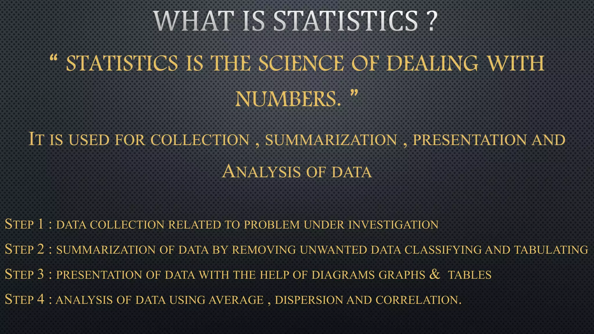
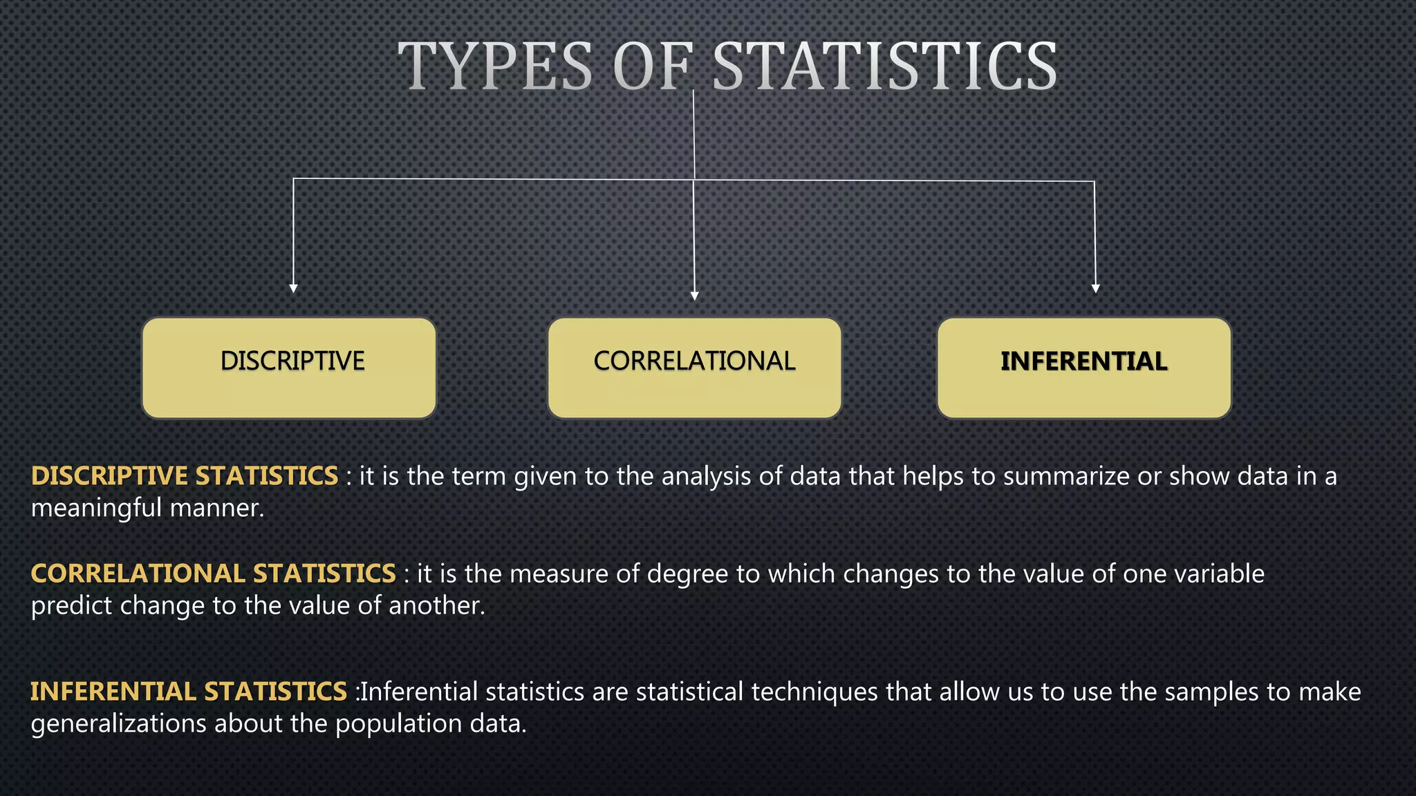
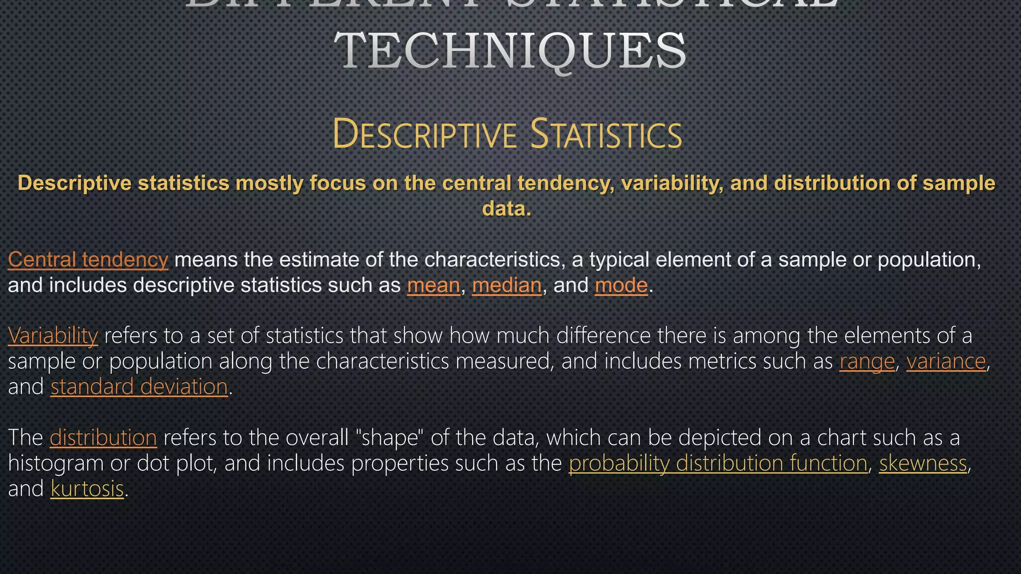
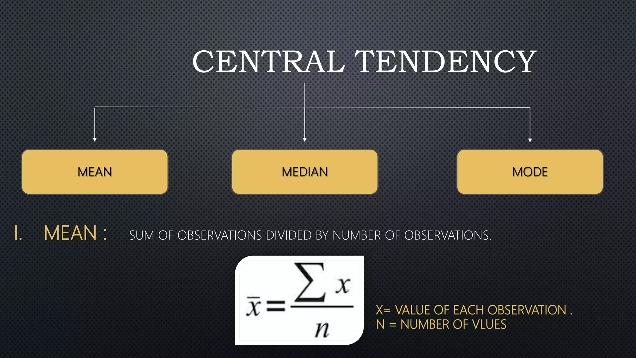
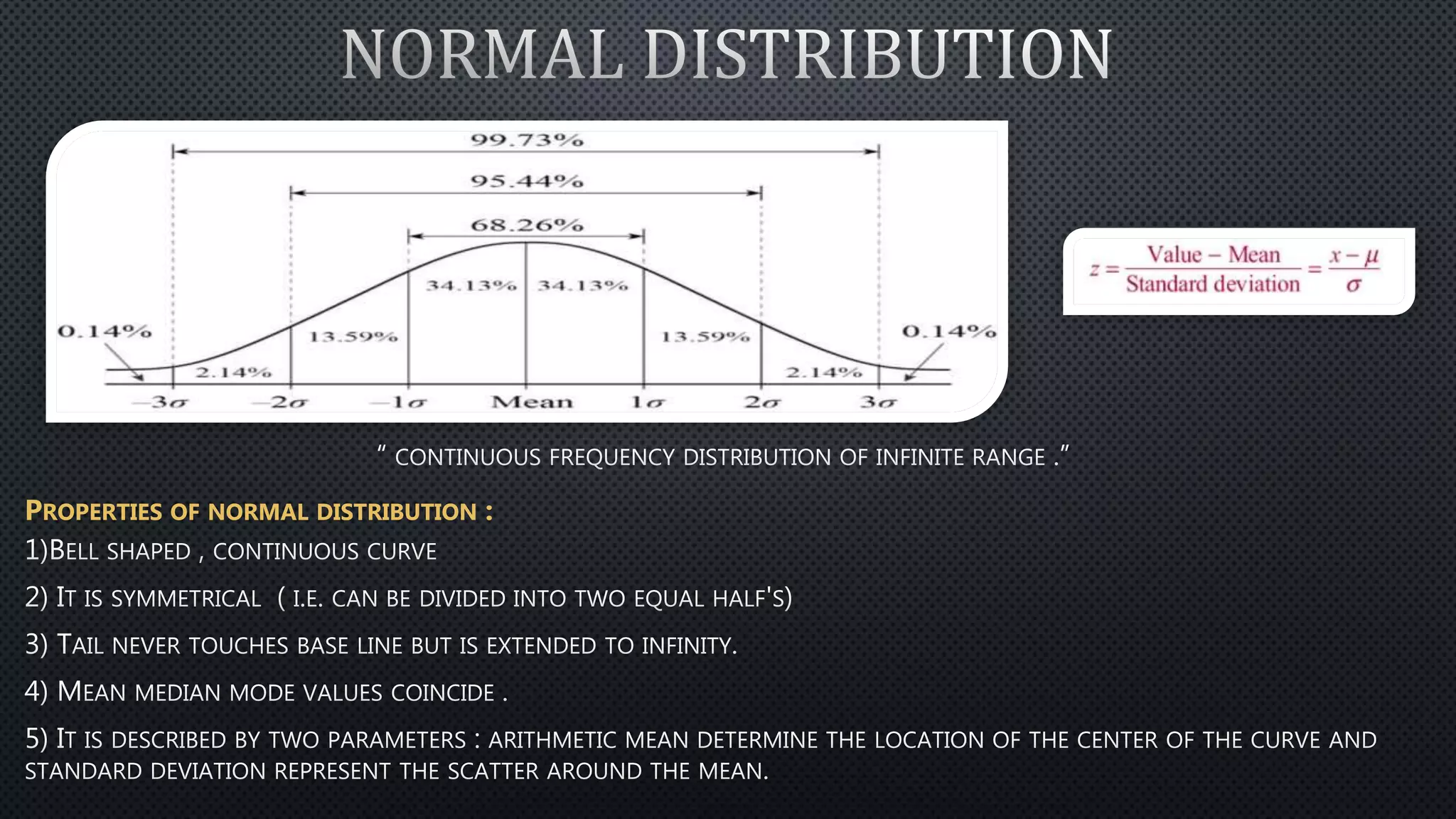
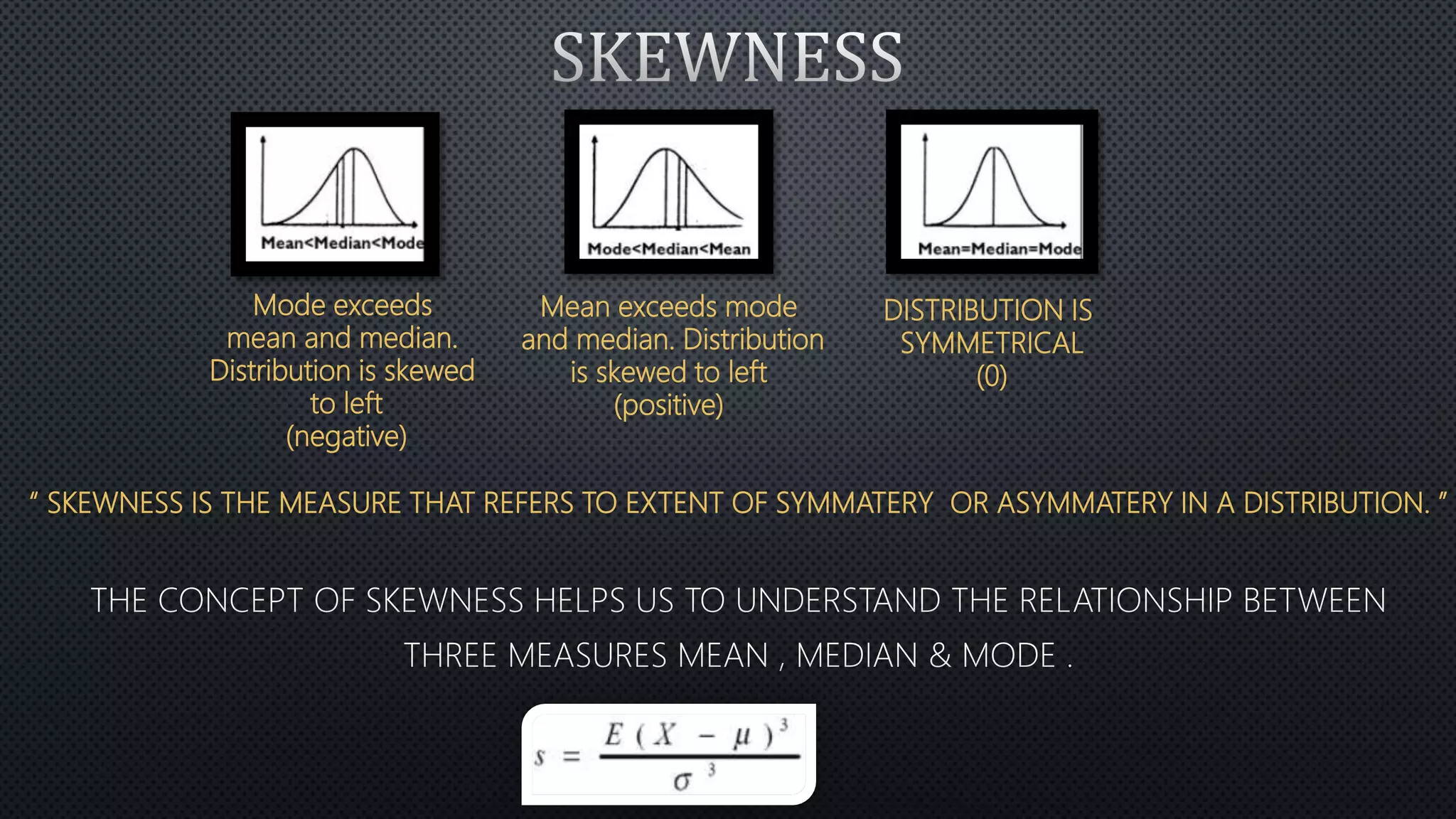
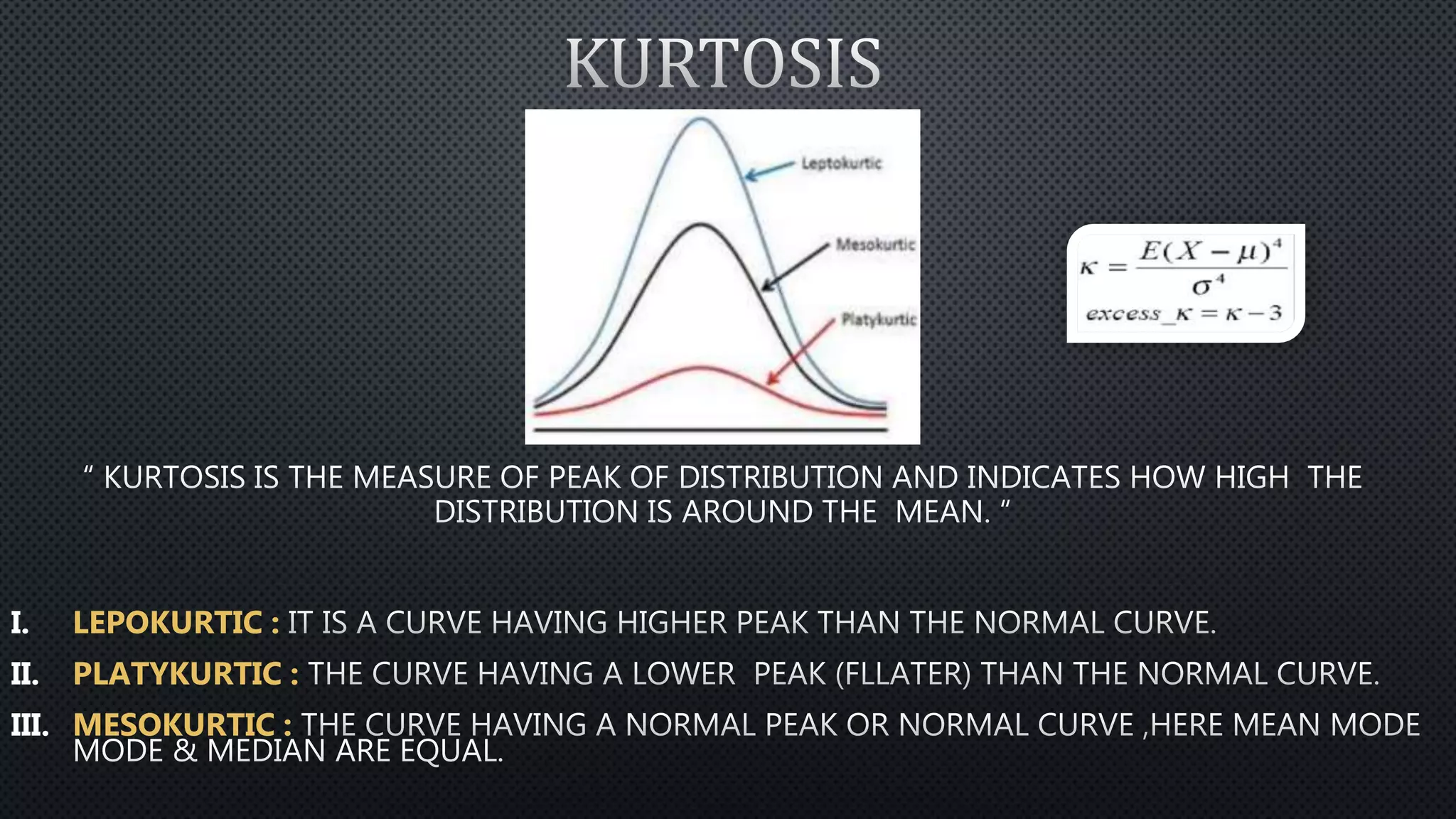
Statistical techniques used in measurement

“ STATISTICS IS THE SCIENCE OF DEALING WITH
NUMBERS. ”
IT IS USED FOR COLLECTION , SUMMARIZATION , PRESENTATION AND
ANALYSIS OF DATA
STEP 1 : DATA COLLECTION RELATED TO PROBLEM UNDER INVESTIGATION
STEP 2 : SUMMARIZATION OF DATA BY REMOVING UNWANTED DATA CLASSIFYING AND TABULATING
STEP 3 : PRESENTATION OF DATA WITH THE HELP OF DIAGRAMS GRAPHS & TABLES
STEP 4 : ANALYSIS OF DATA USING AVERAGE , DISPERSION AND CORRELATION.

INFERENTIAL
DISCRIPTIVE STATISTICS : it is the term given to the analysis of data that helps to summarize or show data in a
meaningful manner.
INFERENTIAL STATISTICS :Inferential statistics are statistical techniques that allow us to use the samples to make
generalizations about the population data.
CORRELATIONAL STATISTICS : it is the measure of degree to which changes to the value of one variable
predict change to the value of another.

QUANTITATIVE DATA : IT IS NUMERICAL DATA.
A) DISCRETE DATA
B) CONTINUOUS DATA
QUALITATIVE DATA : IT IS NON NUMERICAL DATA.
A) CATEGORICAL : DATA IS PURELY DISCRIPTIVE AND IMPLY NO ODERING OF ANY KIND ( SEX,
AREA OF RECIDENCE.)
B) ORDINAL DATA : THOSE WHICH IMPLY SOME KIND OF ODERING (LEVEL OF EDUCATION ,
DEGREE OD SEVERITY OF DISEASE
QUANTITATIVE QUALITATIVE

IN STATISTICS THE TERM MEASUREMENT IS USED MORE BROADLY AND IS MORE
APPROPRIATELY TERMED AS SCALE OF MEASUREMENT.
4 SCALES OF MEASUREMENT ARE :
1. NOMINAL
2. ORDINAL
3. INTERVAL
4. RATIO

CATAGORICAL DATA AND NUMBERS THAT ARE SIMPLY USED AS IDENTIFIRES OR
NAMES REPRESENT A NOMINAL SCALE OF MEASUREMENT
EXAMPLES OF NOMINAL CLASSIFICATION :
1) GENDER
2) NATIONALITY
3) ETHNICITY
4) LANGUAGE
5) STYLE

AN ORDINAL SCALE OF MEASUREMENT REPRESENT THE ORDERED SERIES OF RELATIONSHIPS
OR RANK ORDER.
EXAMPLES OF ORDINAL SCALE :
1) RESULT OF WORLDCUP ( FIRST PLACE , RUNNER-UP , THIRD )
2) MILITARY RANK
3) MEDICAL CONDITION (SATISFACTORY , SERIOUS , CRITICAL )

ARRANGES OBJECTS ACCORDING TO THEIR MAGNITUDES AND DISTINGUISHES THIS ORDERD
ARRANGEMENT IN UNITS OF EQUAL INTERVALS.
EXAMPLES OF INTERVAL SCALE ARE :
1) TIME
2) MEASUREMENT OF SEA LEVEL
3) THE FAHRENHEIT SCALE

THE RATIO SCALE MEASUREMENT IS SIMILAR TO INTERVAL SCALE IN THAT IT ALSO
REPRESENTS QUANTITY AND HAS EQUALITY OF UNITS.
THE EXAMPLES OF RAIO SCALE ARE :
1) MASS
2) ENERGY
3) DURATION
4) LENGTH
5) ELECTRIC CHARGE

DESCRIPTIVE STATISTICS
Descriptive statistics mostly focus on the central tendency, variability, and distribution of sample
data.
Central tendency means the estimate of the characteristics, a typical element of a sample or population,
and includes descriptive statistics such as mean, median, and mode.
Variability refers to a set of statistics that show how much difference there is among the elements of a
sample or population along the characteristics measured, and includes metrics such as range, variance,
and standard deviation.
The distribution refers to the overall "shape" of the data, which can be depicted on a chart such as a
histogram or dot plot, and includes properties such as the probability distribution function, skewness,
and kurtosis.

MEDIAN MODE
MEAN
CENTRAL TENDENCY
I. MEAN : SUM OF OBSERVATIONS DIVIDED BY NUMBER OF OBSERVATIONS.
X= VALUE OF EACH OBSERVATION .
N = NUMBER OF VLUES

AGE OF 5 STUDENTS IS GIVEN 13 ,11, 9 , 10 ,12 FIND MEAN ?
MEAN = (SUM OF OBSERVATIONS )/ (NUMBER OF OBSERVATIONS
SUM OF OBSERVATIONS = 13+11+9+10+12 = 5
NUMBER OF OBSERVATIONS = 5
MEAN = (55)/(5)
=11

II. MEDIAN :
IF NUMBER OF OBSERVATIONS IS ODD
MEDIAN = ( N+1)/2 TERM
IF NUMBER OF OBSERVATIONS IS EVEN
MEDIAN = N / 2 TERM
CALCULATE MEDIAN OF FOLLOWING DATA
4 , 5 , 7 , 8 , 3 , 2 , 4
NUMBER OF TERMS = 7 (ODD)
MEDIAN = (N+1)/2
MEDIAN = (7+1)/2=4
THERE FORE THE FOURTH TERM IS MEDIAN (I.E 8)

III. MODE
CALCULATE MODE FROM THE FOLLOWING DATA
1, 2 ,8, 7 ,8 ,1 ,8 , 2
IN THE ABOVE DATA WE CAN SEE 8 IS REPEATING MAXIMUM NUMBER
OF TIMES SO THIS IS THE MODE

VARIABILITY
I. RANGE :
CALCULATE RANGE FROM THE FOLLOWING DATA
10,3,6,8,1,5,4
RANGE = 10-1=9
RANGE VARIENCE STANDERD DEVIATION

II. VARIENCE :
I.
II.
III.
IV.
V.
N= NUMBER OF TERMS
X= OBSERVATION VALUE

III. STANDARD DEVIATION :
I. FIND MEAN OF THE DATA
II. SUBTRACT MEAN FROM EACH VALUE- THE RESULT IS CALLED THE DEVIATION FROM MEAN
III. SQUARE EACH DEVIATION FROM MEAN.
IV. FIND SUM OF THE SQUARES.
V. DIVIDE THE TOTAL BY NUMBER OF ITEMS
VI. TAKE THE UNDER ROOT OF THIS.
UNDER ROOT OF VARIENCE
IT IS DENOTED BY “ SIGMA “

I. PROBABILITY DISTRIBUTION FUNCTION
PROBABILITY
DISTRIBUTION
FUNCTION
SKEWNESS KURTOSIS
DISCRETE CONTINUOUS

A) DISCRETE DISTRIBUTION
CONTINUOUS DISTRIBUTION :
3 TYPES OF CONTINUOUS DISTRIBUTION :
•
•
•

PROPERTIES OF NORMAL DISTRIBUTION :

“ SKEWNESS IS THE MEASURE THAT REFERS TO EXTENT OF SYMMATERY OR ASYMMATERY IN A DISTRIBUTION. ”
Mode exceeds
mean and median.
Distribution is skewed
to left
(negative)
Mean exceeds mode
and median. Distribution
is skewed to left
(positive)
DISTRIBUTION IS
SYMMETRICAL
(0)

I. LEPOKURTIC :
II. PLATYKURTIC :
III. MESOKURTIC :

INFERENTIAL STATISTICS
HYPOTHESIS TESTING
EXAMPLE:
INFERENTIAL STATISTICS ARE STATISTICAL TECHNIQUES THAT ALLOW US TO USE THE SAMPLES TO MAKE
GENERALIZATIONS ABOUT THE POPULATION DATA.

STEPS FOR HYPOTHESIS TESTING
•
•
•
•
TYPES OF HYPOTHESIS TESTING
NULL HYPOHESIS
(No)
ALTERNATIVE
HYPOTHESIS(Na)
1. NULL HYPOTHESIS (No) : A statement about the population parameter.
We test the likelihood of the statement being true in order to decide whether to accept of reject our alternative
hypothesis.
Can include =, < ,> signs

2. ALTERNATIVE HYPOTHESIS(NA)
EXAMPLE :
NULL HYPOTHESIS :
ALTERNATIVE HYPOTHESIS :

METHOD OF ACCESSING THE HYPOTHESIS TESTING IS CALLED SIGNIFICANCE TEST
THE SIGNIFICANCE TESTING :
STEPS OF SIGNIFICANCE TEST :
•
•
•
•
•
•
•

THE SELECTION TEST OF SIGNIFICANCE DEPENDS ESSENTIALLY ON TYPE OF DATA WE HAVE.
QUANTITATIVE DATA QUALITATIVE DATA
T TEST
ANOVA Z TEST
CHI

GENERAL EQUATION FOR T TEST
The applicable number of degrees of freedom here is: df = n-1
When using the t-test for two small sets of data (n1 and/or n2<30), a choice of the type of test must be made
depending on the similarity (or non-similarity) of the standard deviations of the two sets. If the standard deviations
are sufficiently similar they can be "pooled" and the Student t-test can be used. When the standard deviations are
not sufficiently similar an alternative procedure for the t-test must be followed in which the standard deviations are
not pooled. A convenient alternative is the Cochran variant of the t-test.

1) STUDENTS T TEST
EQUATION FOR STUDENT T TEST ( CONVERTED FROM GENERAL T TEST EQUATION )
The pooled standard deviation sp is calculated by:
s1 = standard deviation of data set 1
n1 = number of data in set 1
n2 = number of data in set 2.
the applicable number of degrees of freedom df is here calculated by: df = n1 + n2 -2

COCHRAN'S T-TEST
THE COCHRAN VARIANT OF THE T-TEST IS USED WHEN THE STANDARD DEVIATIONS OF THE
INDEPENDENT SETS DIFFER SIGNIFICANTLY.
To be applied to small data sets (n1, n2, < 30) where s1 and s2, are dissimilar.
Calculate t with:
n1 = number of data in set 1
n2 = number of data in set 2.
¯x1 = mean of data set 1
¯x2 = mean of data set 2
Then determine an "alternative" critical t-value:
t1
= ttab at n1-1 degrees of freedom
t2
= ttab at n2-1 degrees of freedom
NOW THE T-TEST CAN BE PERFORMED AS USUAL: IF TCAL< TTAB
* THEN THE NULL HYPOTHESIS THAT THE
MEANS DO NOT SIGNIFICANTLY DIFFER IS ACCEPTED.

) PAIRED T-TEST
MATCHED SAMPLES IN WHICH INDIVISUALS ARE MATCHED ON PERSONAL
CHARACTERSTICS SUCH AS AGE AND SEX.
STEPS :
1. CALCULATE THE DIFFERENCE (DI = XI – YI) BETWEEN TWO OBSERVATION ON EACH PAIR.
2. CALCULATE MEAN DIFFERENCE D.
3. CALCULATE STANDARD ERROR OF MEAN DIFFERENCES S.E = S.D/(N)^(1/2).
4. CALCULATE T-STATISTIC WHICH IS GIVEN BY T =D/S.E UNDER NULL HYPOTHESIS , THIS STATIC FOLLOWS A
DISTRIBUTION WITH N-1 DEGREE OF FREEDOM.
5. USE TABLES OF T-DISTRIBUTION TO COMPARE YOUR VALUE FOR T TO THE TN-1 DISTRIBUTION . THIS WILL
THE P VALUE FOR THE PAIRED-T TEST.

Example :
Total-P contents (in mmol/kg) of plant tissue as determined by 123 laboratories (Median) and Laboratory L.
¯d = 7.70 tcal =1.21 sd = 12.702
ttab = 3.18
To verify the performance of the laboratory a paired t-test can be performed:
Noting that m d=0 (hypothesis value of the differences, i.e. no difference), the t value can be calculated as:
The calculated t-value is below the critical value of 3.18 (Appendix 1, df = n - 1 = 3, two-sided), hence the null
hypothesis that the laboratory does not significantly differ from the group of laboratories is accepted, and the results of
Laboratory L seem to agree with those of "the rest of the world"

ANALYSIS OF VARIANCE (ANOVA) IS A METHOD FOR TESTING THE HYPOTHESIS THAT THERE IS NO DIFFERENCE BETWEEN
TWO OR MORE POPULATION MEAN.
1)
2)
1) ONE-WAY ANALYSIS
2) TWO-WAY ANALYSIS

A practical quantification of the uncertainty is obtained by calculating the standard deviation of the points
on the line; the "residual standard deviation" or "standard error of the y-estimate", which we assumed to be
constant
n = number of calibration points.
= "fitted" y-value for each xi, (read from graph or calculated with Eq. 6.22).
is the (vertical) deviation of the found y-values from the line.
Only the y-deviations of the points from the line are considered. It is assumed that deviations in the x-direction are
negligible. This is, of course, only the case if the standards are very accurately prepared.
Now the standard deviations for the intercept a and slope b can be calculated with:
and
The uncertainty about the regression line is expressed by the confidence limits of a and b : a ± t.sa and b ± t.sb

Example: In the present example
and,
and,
The applicable ttab is 2.78 (App. 1, two-sided, df = n -1 = 4) hence
a = 0.037 ± 2.78 × 0.0132 = 0.037 ± 0.037
and
b = 0.626 ± 2.78 × 0.0219 = 0.626 ± 0.061

QUALITATIVE DATA ARE ARRANGED IN TABLE FORMED BY ROWS AND COLUMNS , ONE VARIABLE DEFINE THE
ROWS AND OTHER VARIABLE DEFINE THE COLUMN.
IT IS DENOTED BY GR. SIGN-
DEGREE OF FREEDOM (F) = (ROW-1) (COLUMN-1)
E(EXPECTED VALUE) IS CALCULATED BY : [ TOTAL ROW X TOTAL COLUMN / GRAND TOTAL]
( RT X CT / GT )
O = observed value in table
E = expected value in table

Z TEST IS A STATISTICAL PROCEDURE USED TO TEST AN ALTERNATIVE HYPOTHESIS AGAINST A NULL HYPOTHESIS.
FORMULA FOR VALUE OF Z (IN Z-TEST):
FORMULA FOR Z FOR COMPARING TWO PERCENTAGES :
P1= PERCENTAGE IN THE 1ST GROUP
P2 = PERCENTAGE IN THE 2ND GROUPR
Q1=100-P1 Q2=100-P2 N1= SAMPLE SIZE OF GROUP 1
N2= SAMPLE SIZE OF GROUP 2

THE F-TEST (OR FISHER'S TEST) IS A COMPARISON OF THE SPREAD OF TWO SETS OF DATA TO TEST IF THE SETS
BELONG TO THE SAME POPULATION, IN OTHER WORDS IF THE PRECISIONS ARE SIMILAR OR DISSIMILAR.
where the larger s2 must be the numerator by convention. If the performances are not very different, then the estimates s1, and s2, do not
differ much and their ratio (and that of their squares) should not deviate much from unity. In practice, the calculated F is compared with the
applicable F value in the F-table (also called the critical value, see Appendix 2). To read the table it is necessary to know the applicable
number of degrees of freedom for s1, and s2. These are calculated by:
df1 = n1-1
df2 = n2-1
If Fcal  Ftab one can conclude with 95% confidence that there is no significant difference in precision (the "null
hypothesis" that s1, = s, is accepted). Thus, there is still a 5% chance that we draw the wrong conclusion. In certain
cases more confidence may be needed, then a 99% confidence table can be used, which can be found in statistical
textbooks.

Statistical techniques used in measurement

Statistical techniques used in measurement

More Related Content

What's hot

Similar to Statistical techniques used in measurement

Recently uploaded

Statistical techniques used in measurement