Download to read offline
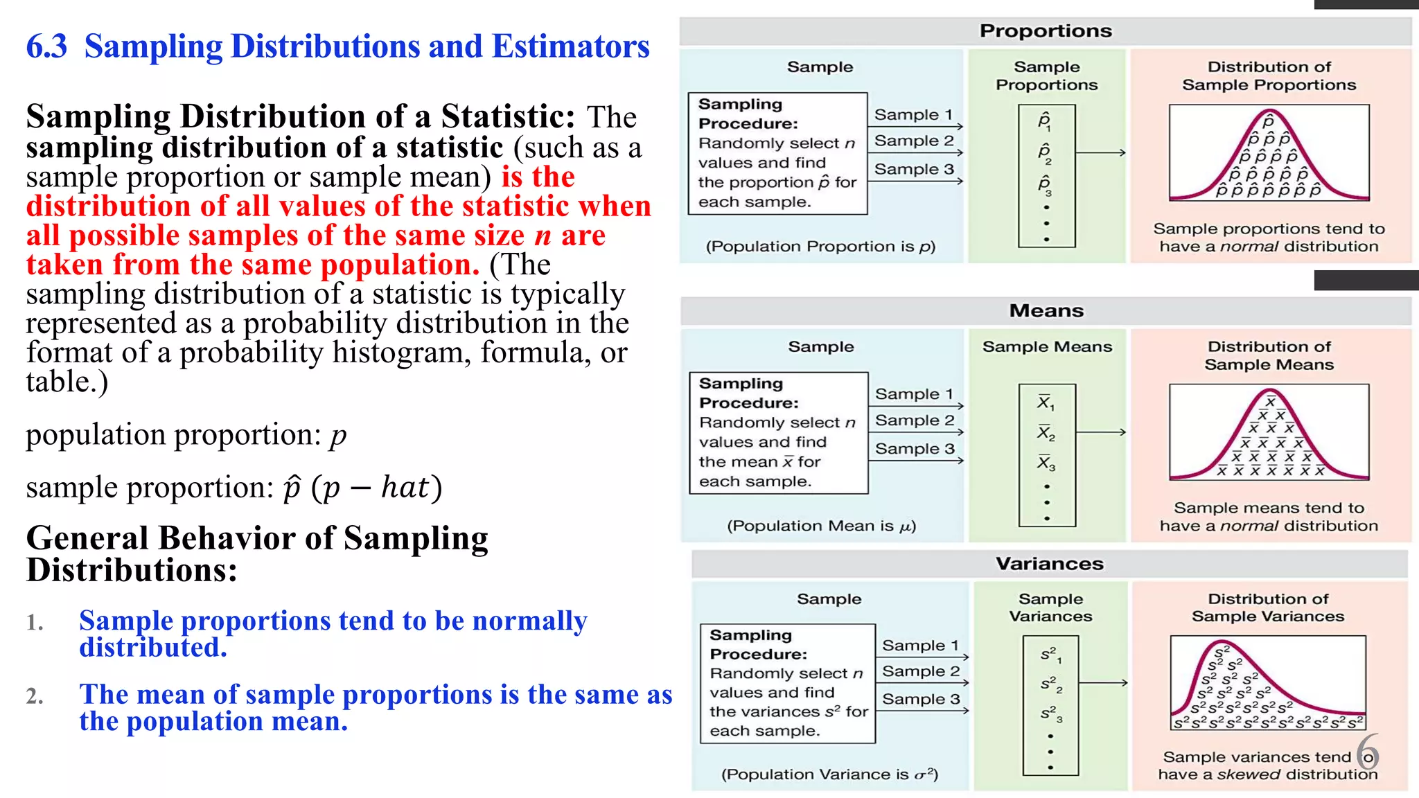


The document discusses sampling distributions and estimators from chapter 6 of an elementary statistics textbook. It defines a sampling distribution of a statistic as the distribution of all values of a statistic (such as sample mean or proportion) obtained from samples of the same size from a population. The sampling distributions of sample proportions and means tend to be normally distributed, with their means converging on the population parameter. Specifically, the mean of sample proportions equals the population proportion, and the mean of sample means equals the population mean. The distribution of sample variances, on the other hand, tends to be right-skewed.
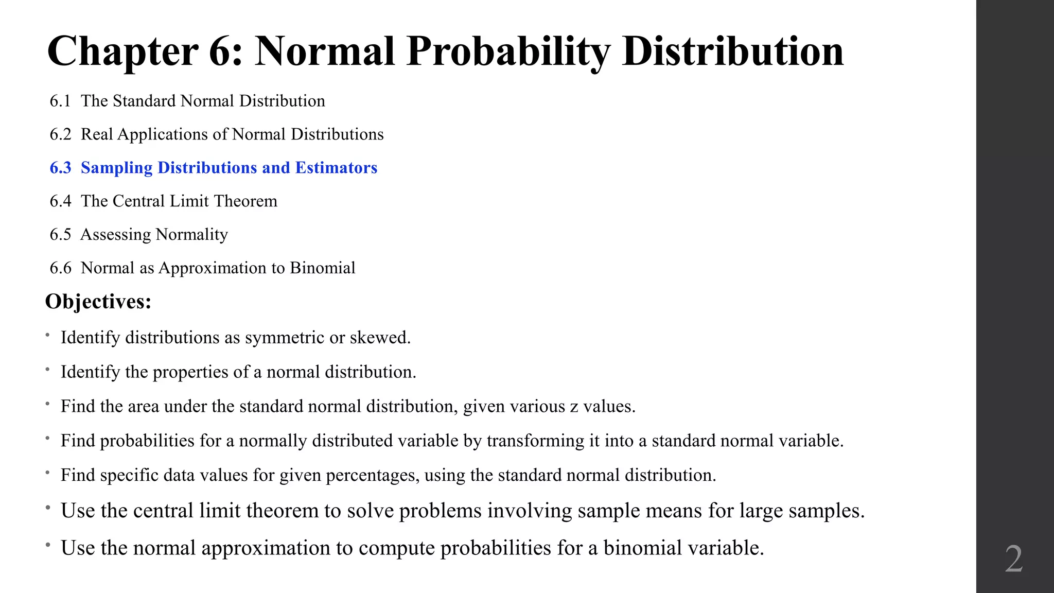
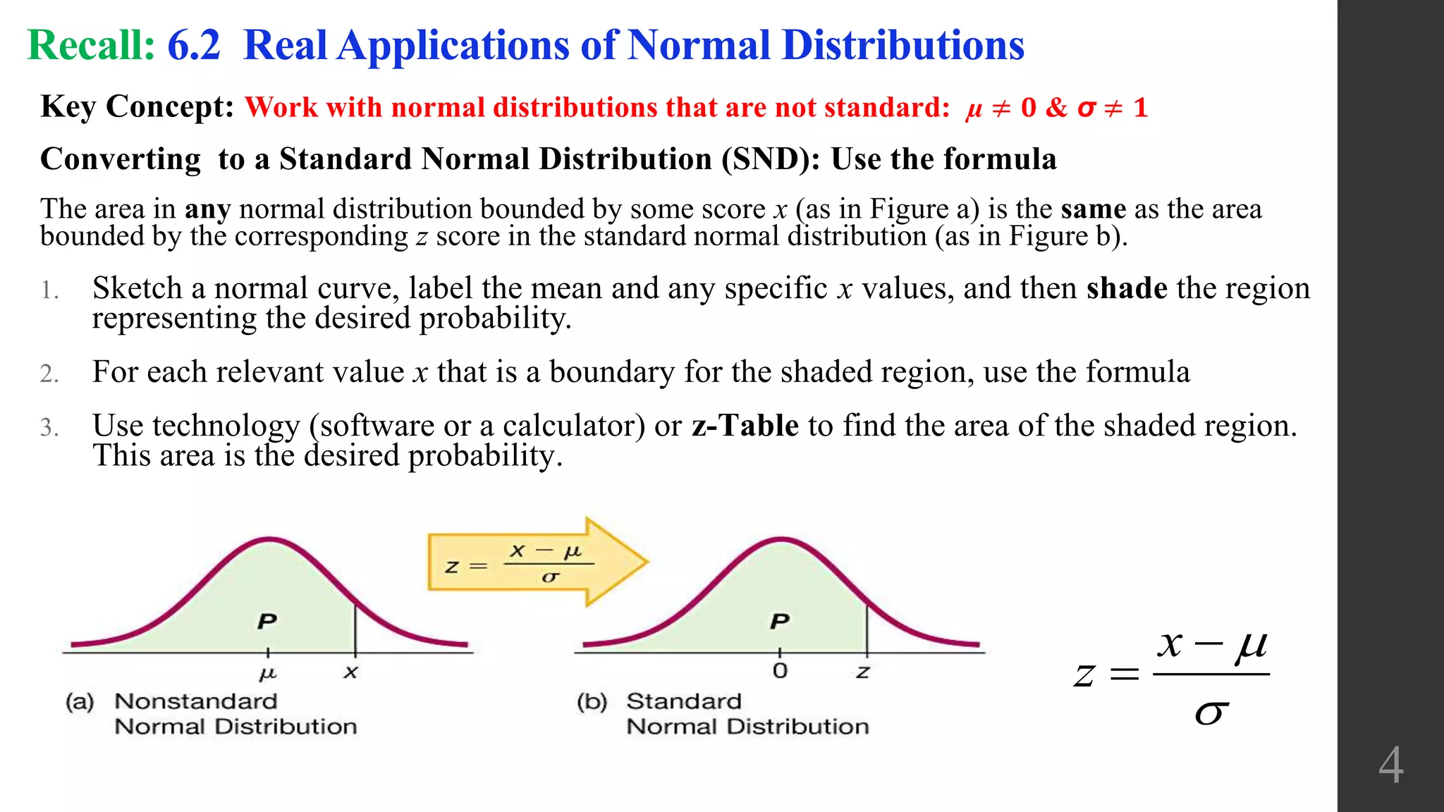
Overview of Normal Probability Distributions including standard normal distribution, applications, objectives, and key concepts.
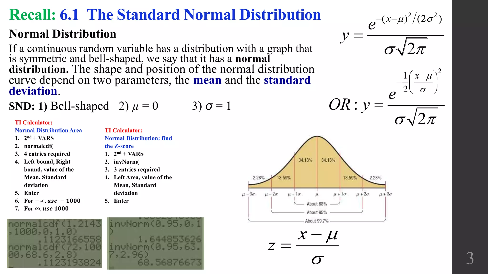
Explanation of normal distributions characteristics, parameters, and converting to standard normal using a TI calculator.
Introduction to sampling distributions focusing on sample means and proportions, their behavior and characteristics.
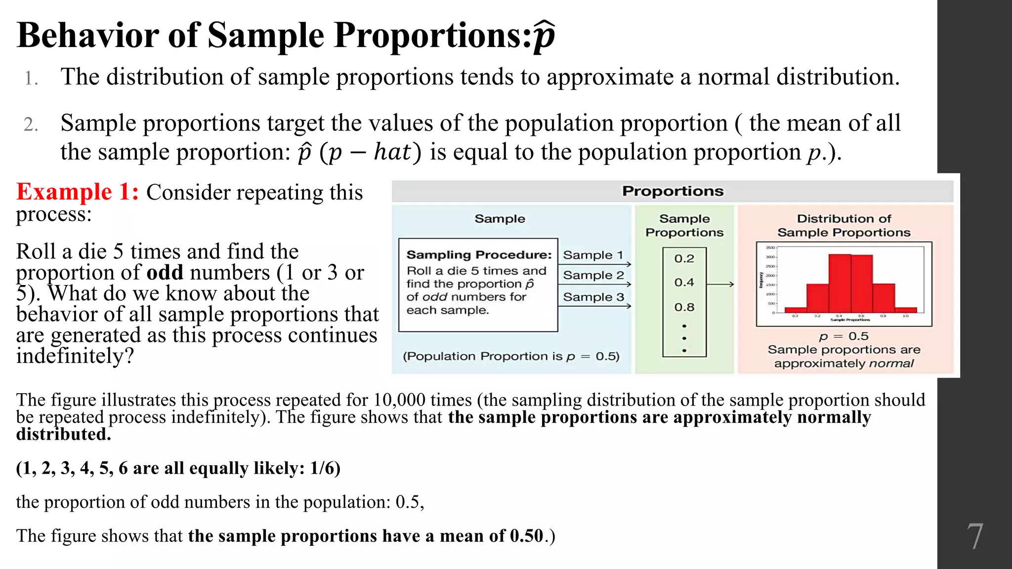
Discussion on how sample proportions approximate a normal distribution with example of rolling a die and its implications.
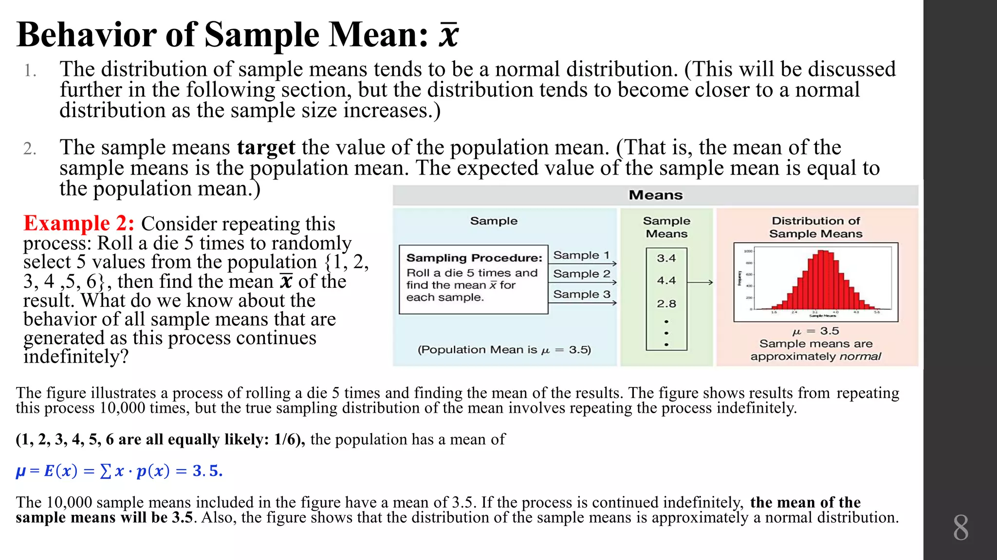
Illustration of sample means behavior through repeated processes, showcasing the convergence towards normal distribution.
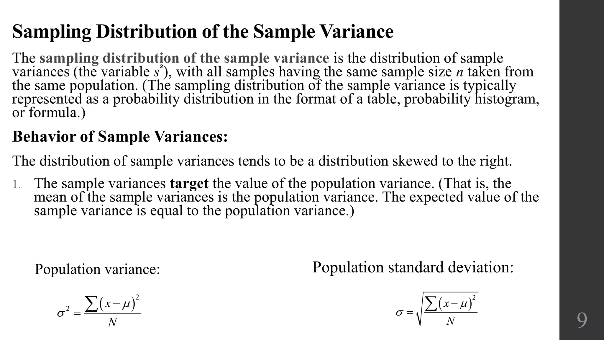
Exploration of the distribution of sample variances, its character, and its targeting of the population variance.