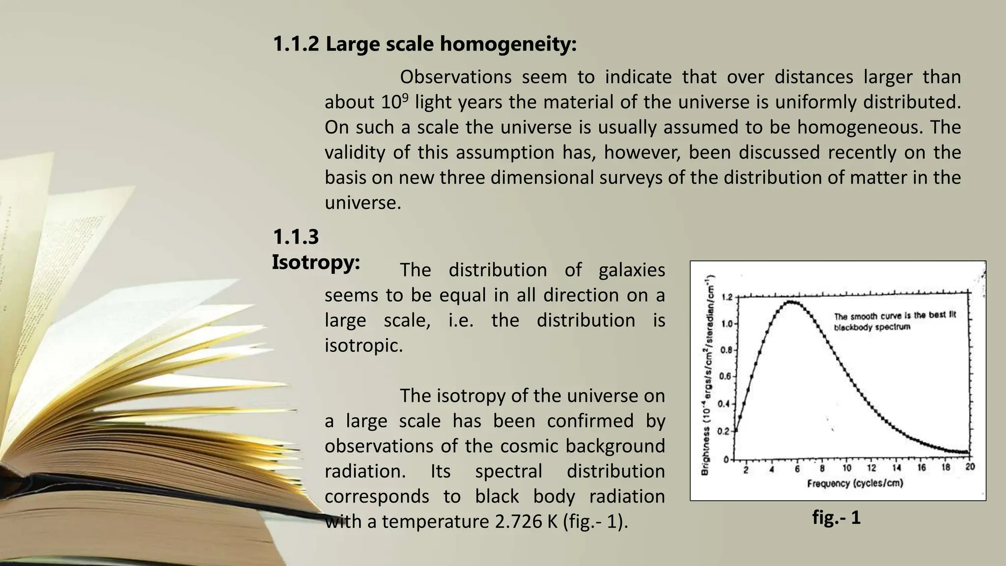
The document discusses the Robertson-Walker metric and its application to cosmological redshifts. It contains the following key points:
1. The Robertson-Walker metric describes a homogeneous and isotropic universe and can account for the observed redshift of distant galaxies by considering the expansion of the universe over time.
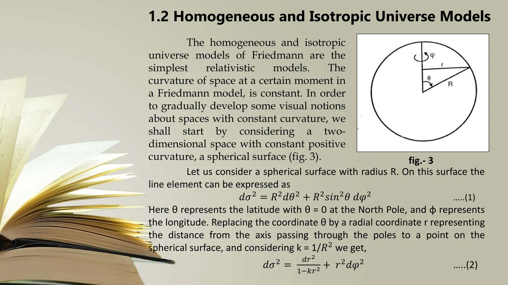
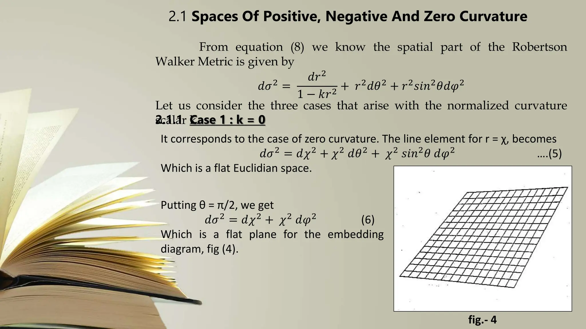
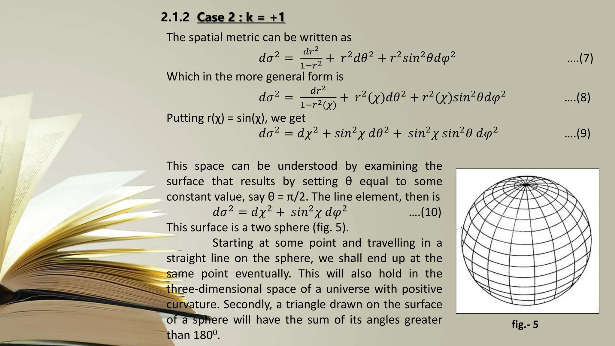
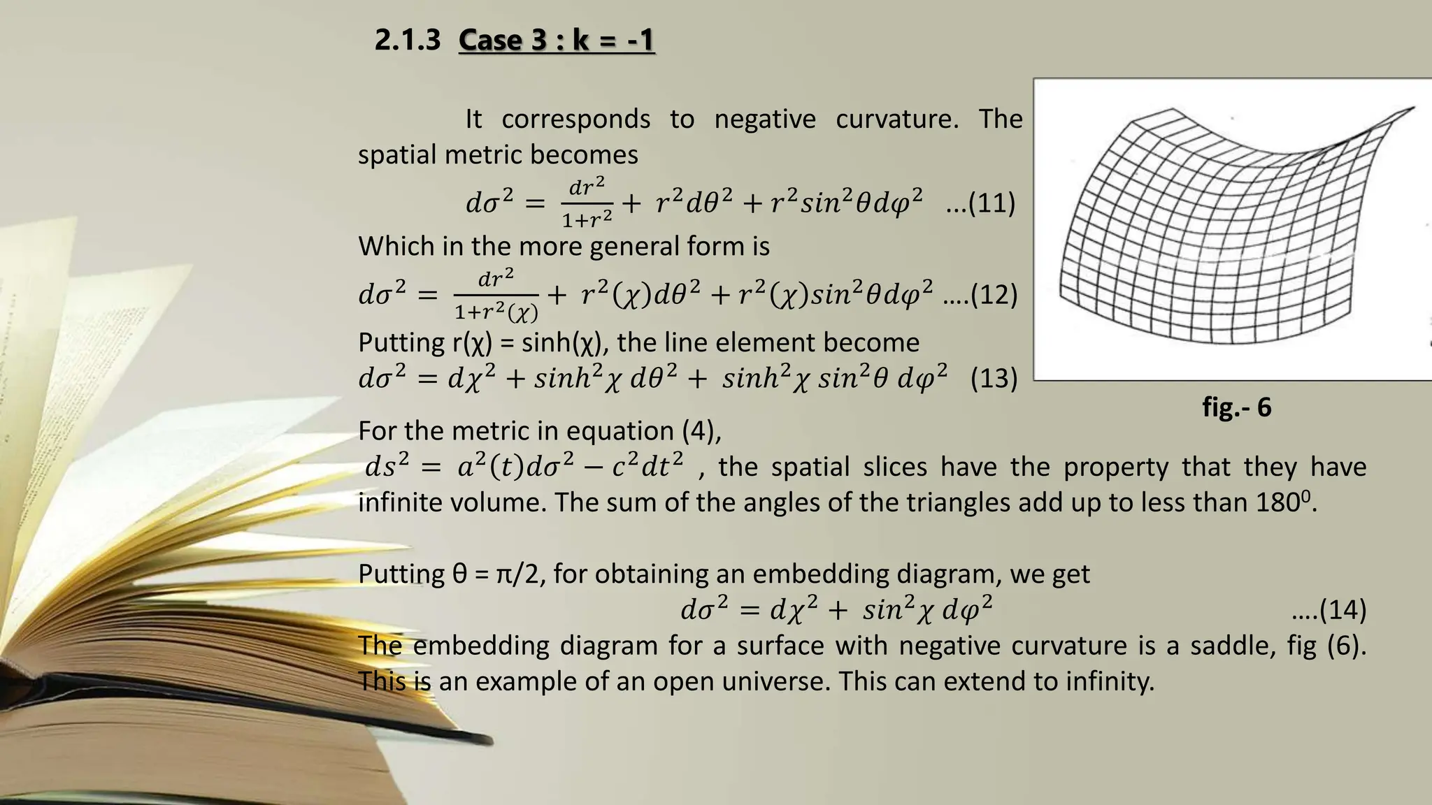
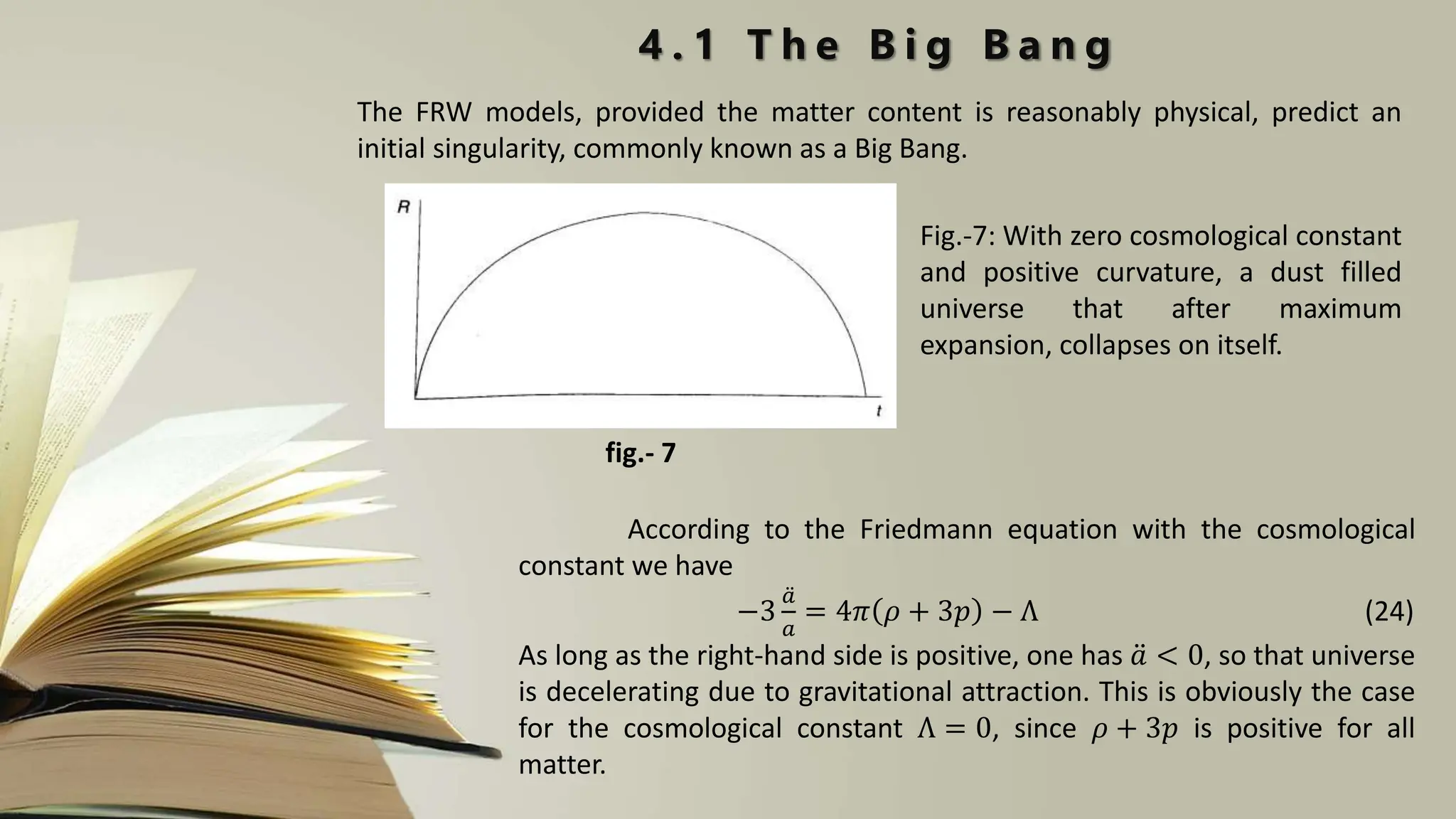
2. The metric allows for spaces with positive, negative, or zero curvature, corresponding to closed, open, or flat geometries for the universe.
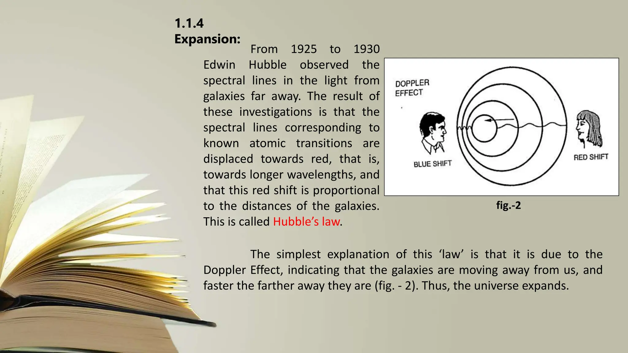
3. Application of the metric successfully explains Hubble's observation of redshift proportional to distance as being due to the Doppler effect from the receding motion of galaxies caused by the expansion of the universe.