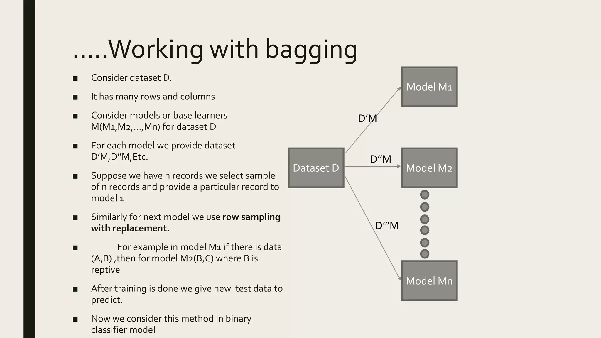
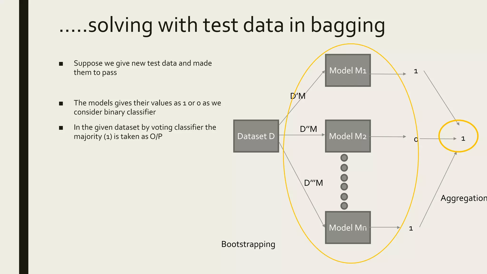
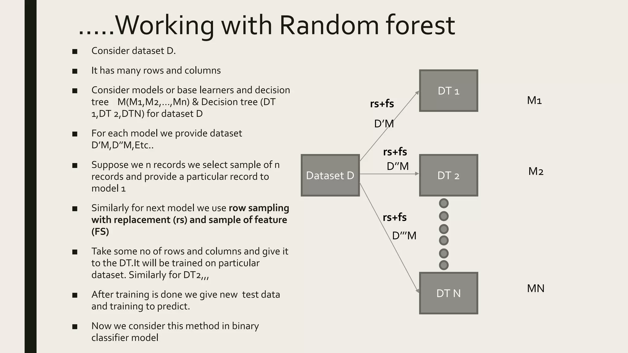
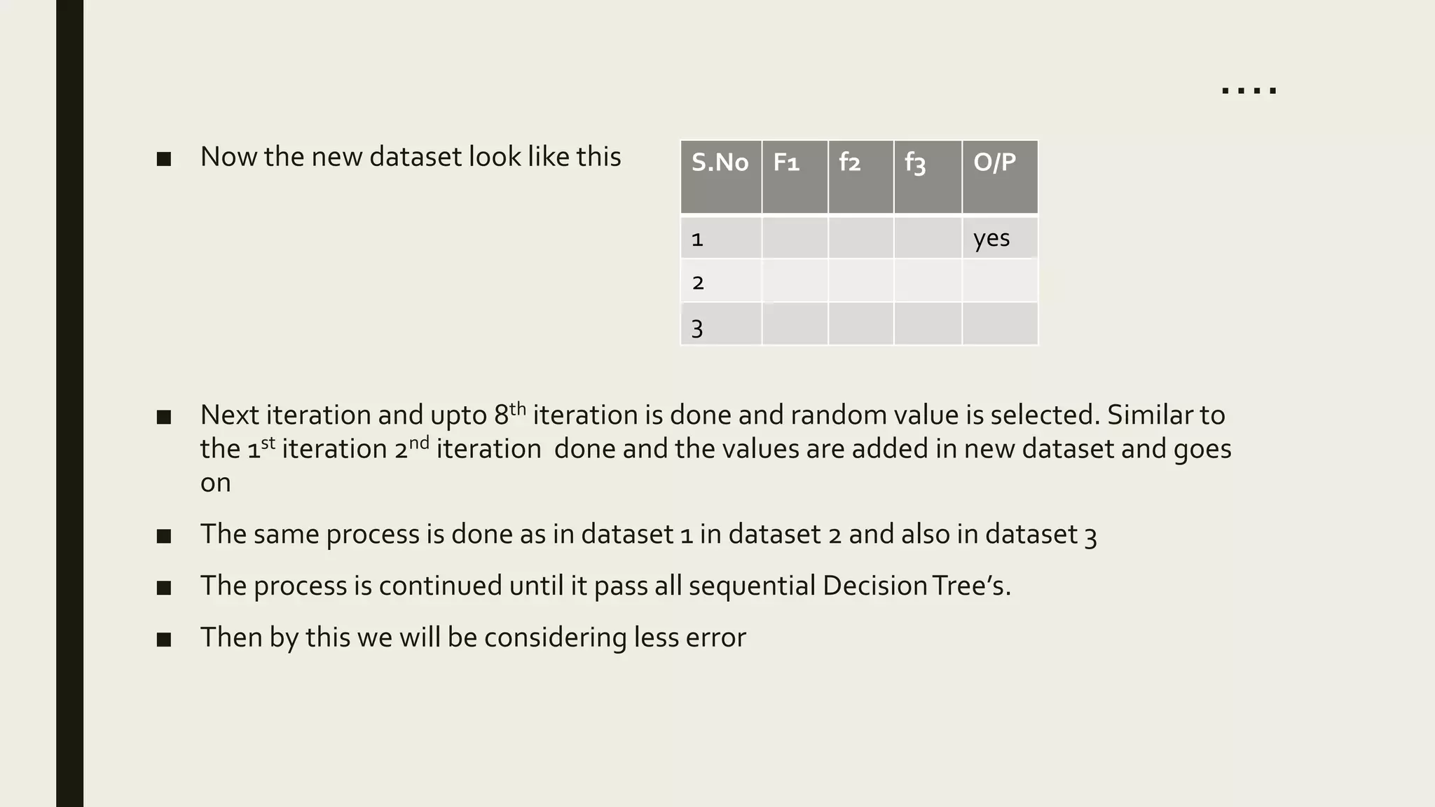
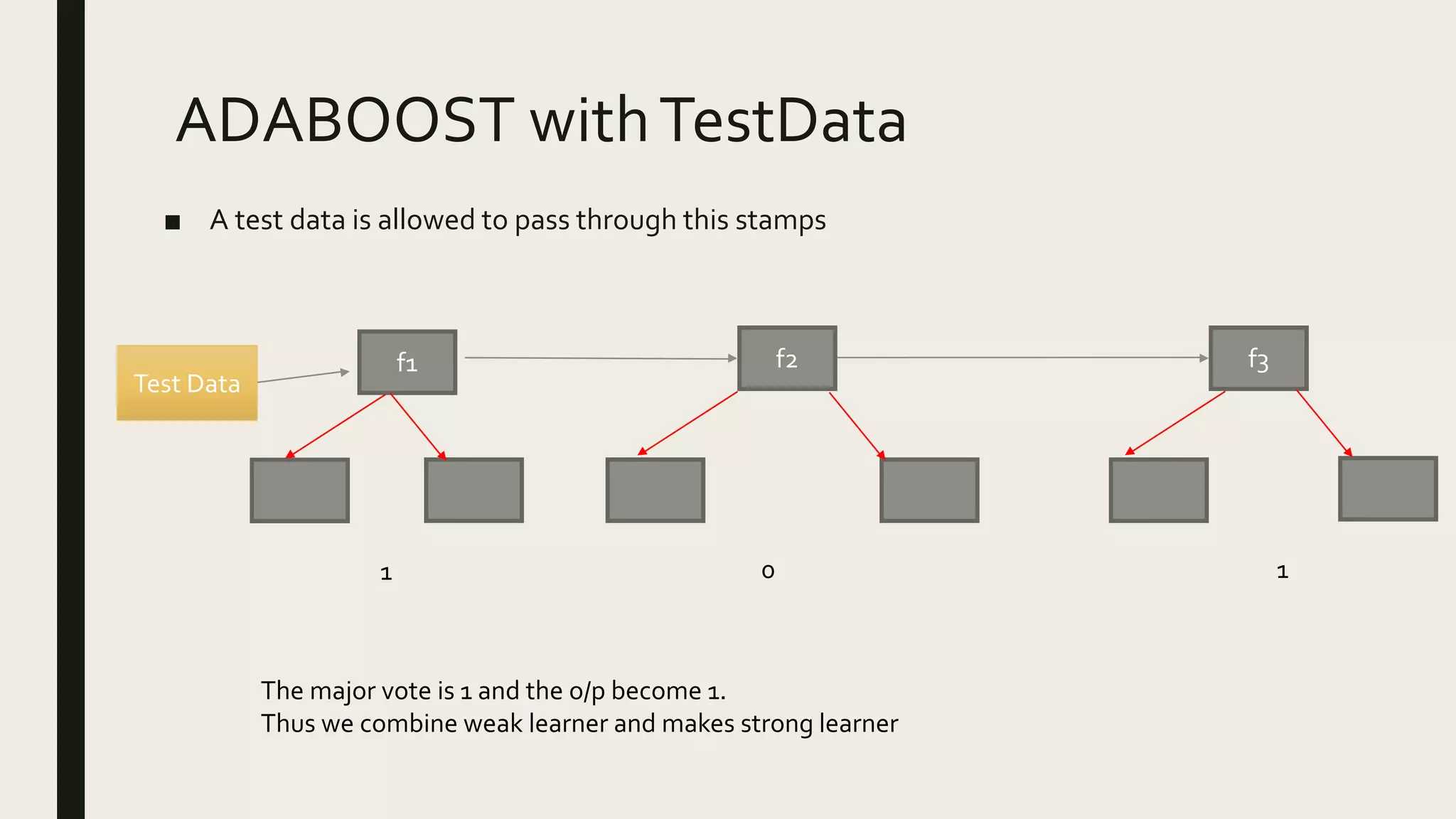
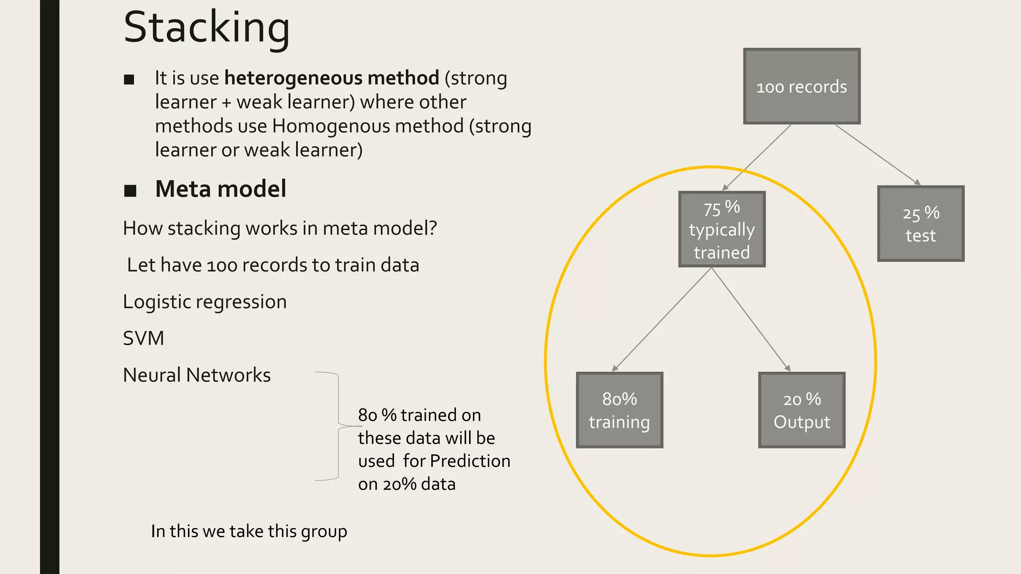
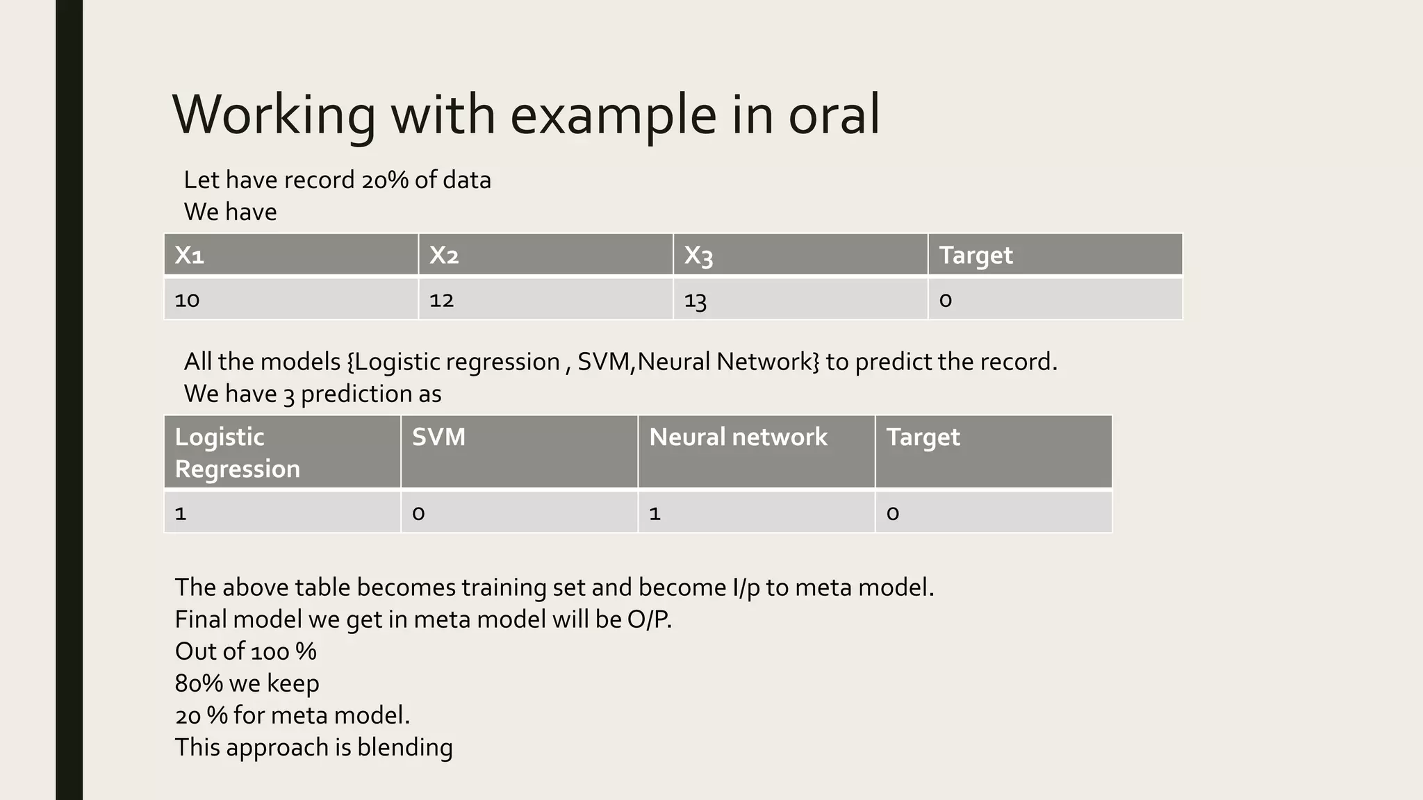
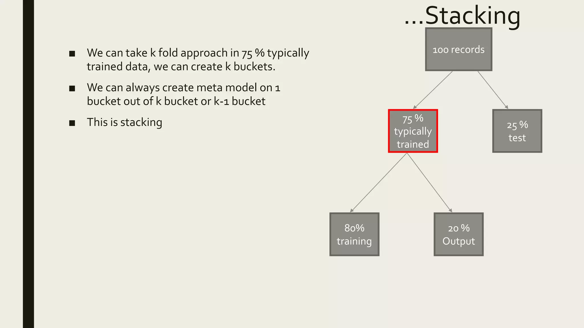
ENSEMBLE
METHODS
Why do we use Ensemble methods ?
■ Ensemble learning helps improve machine learning results
by combining several models.
■ This approach allows the production of better predictive
performance compared to a single model
■ Ensemble methods are meta-algorithms that combine
several machine learning techniques into one predictive
model in order
to decrease variance (bagging), bias (boosting),
or improve predictions (stacking).
Groups
■ Sequential Ensemble methods where the base learners are
generated sequentially (e.g. AdaBoost).
■ Parallel Ensemble methods where the base learners are
generated in parallel (e.g. Random Forest).
Methods
■ Bagging
■ Random Forest
■ Boosting
■ Adaptive Boost (Adaboost)
■ Stacking
Bagging
■ Bagging stands for bootstrap aggregation.
■ One way to reduce the variance of an estimate
is to average together multiple estimates.
…..Working with bagging
■ Consider dataset D.
■ It has many rows and columns
■ Consider models or base learners
M(M1,M2,…,Mn) for dataset D
■ For each model we provide dataset
D’M,D’’M,Etc.
■ Suppose we have n records we select sample
of n records and provide a particular record to
model 1
■ Similarly for next model we use row sampling
with replacement.
■ For example in model M1 if there is data
(A,B) ,then for model M2(B,C) where B is
reptive
■ After training is done we give new test data to
predict.
■ Now we consider this method in binary
classifier model
Dataset D
Model Mn
Model M2
Model M1
D’M
D’’M
D’’’M
…..solving with test data in bagging
■ Suppose we give new test data and made
them to pass
■ The models gives their values as 1 or 0 as we
consider binary classifier
■ In the given dataset by voting classifier the
majority (1) is taken as O/P Dataset D
Model Mn
Model M2
Model M1
D’M
D’’M
D’’’M
1
1
0 1
Bootstrapping
Aggregation
Random Forest
■ One of the technique used for bagging is random
forest
■ Random Forest models decide where to split
based on a random selection of features. Rather
than splitting at similar features at each node
throughout, Random Forest models implement a
level of differentiation because each tree will split
based on different features.
…..Working with Random forest
■ Consider dataset D.
■ It has many rows and columns
■ Consider models or base learners and decision
tree M(M1,M2,…,Mn) & Decision tree (DT
1,DT 2,DTN) for dataset D
■ For each model we provide dataset
D’M,D’’M,Etc..
■ Suppose we n records we select sample of n
records and provide a particular record to
model 1
■ Similarly for next model we use row sampling
with replacement (rs) and sample of feature
(FS)
■ Take some no of rows and columns and give it
to the DT.It will be trained on particular
dataset. Similarly for DT2,,,
■ After training is done we give new test data
and training to predict.
■ Now we consider this method in binary
classifier model
Dataset D
DT N
DT 2
DT 1
D’M
D’’M
D’’’M
M1
MN
M2
rs+fs
rs+fs
rs+fs
…..Working with Random forest
■ Suppose we give new test data and made
them to pass
■ The models gives their values as 1 or 0 as we
consider binary classifier
■ In the given dataset by voting classifier the
majority (1) is taken as O/P
Dataset D
DT N
DT 2
DT 1
D’M
D’’M
D’’’M
M1
MN
M2
rs+fs
rs+fs
rs+fs
1
0
1
1
Why do we use Random forest for
decision tree?
Decision tree basically has
Low Bias –When we are training a DecisionTree to its complete depth,then it will be properly
trained so training error is less
HighVariance –When we give new test data ,it give larger amount of error in it so
there occurs a high variance.
In random forest we use multiple Decision tree and we know it has high variance but when we
combine all decision tree with respect to majority vote,the high variance will be reduced to low
variance
When we are sampling and giving records to decision tree ,the decision tree tends to become
expert with respect to rows.
In this way the high variance is converted to low variance
Advantage with example
■ Suppose we have 1000 records they get
spilted into decision trees.
■ Now if we give 200 records as new data
they does not create a great impact in it
Dataset D
DT N
DT 2
DT 1
D’M
D’’M
D’’’M
M1
MN
M2
rs+fs
rs+fs
rs+fs
1
0
1
1
Regressor
■ If we use regression instead of binary
classifier, we use this method as
■ It takes the average value
Dataset D
DT N
DT 2
DT 1
D’M
D’’M
D’’’M
M1
MN
M2
rs+fs
rs+fs
rs+fs
2000
1000
3000
2000
Important Note
Classifier is solved by Major vote
Regressor is solved by average of votes
Boosting
■ Boosting refers to a family of algorithms that are able
to convert weak learners to strong learners.
■ The predictions are then combined through a
weighted majority vote (classification) or a weighted
sum (regression) to produce the final prediction.
Working with Boosting
■ Consider a dataset with records
■ Consider models(M1,M2,..,Mn) or
base learners
■ Some data are passed to base learners
or model once it is trained .
■ After training we will pass records to
base learners or model and see how
particular model is performed
Dataset
Records
M1
M2
Mn
..cont
■ The records are allowed to pass to
model M1 and red coloured 2
records are incorrectly classified,
the next model will be created
sequentially and only 2 records
will be passed to next model M2
■ If M2 gives some wrong records
then the error will be passed
continuously to M3
■ This will go until we specify some
strong learners.
■ This boosting technique will make
weak learners to strong learners.
M1
M2
Mn
ADABOOST or ADAptive BOOSTing
■ It is little different.
■ There is something called weights will be assigned here.
■ Suppose we have features and O/P
There are 5 Steps we need to do .They are
Step 1 - Calculate Sample weight
Step 2 – Create 1st base learner
Step 3 – Find the performance of stamp
Step 4 – Updating Sample weight
Step 5 - Calculating normalized weight
Step 1 - Calculate Sample weight
Sample weight(w)=1/n
here n = 7(since 7 records)
so sample weight(w)=1/7
All records contains same sample
weight as 1/7
S.No F1 f2 f3 O/P Sample weight
(W)
1 1/7
2 1/7
3 1/7
4 1/7
5 1/7
6 1/7
7 1/7
Step 2 – Create 1st base learner
■ We will create with the help Decision tree in AdaBoost.
■ In this decision tree is not created as in random forest
■ It is created with help of stamps (Stamps are one that has 1 depth in tree)
■ Let us consider 3 stamps with our functions
■ We consider function f1 and create stamp and sequentially for f2,f3 as shown
f1 f2 f3
…
■ From the 1st decision tree we have to
create Base learners model
■ Compare f1,f2,f3 & select base learners
model
■ Consider Binary classifier as
Output(Yes/No)
■ If we select f1 as Base learners model .
■ If there are 6 records correctly classified
and 1 record is incorrectly classified ,we
have to find total error for that
incorrectly classified one(red colour
marked).Total error is calculated by
summing up sample weight.
Since there is one row has error
,the sample weight is taken with
that,
Total error = (1/7)+0(since no
other record causes errors)
=(1/7)
S.No F1 f2 f3 O/P Sample
weight
1 Yes 1/7
2 No 1/7
3 Yes 1/7
4 Yes 1/7
5 No 1/7
6 No 1/7
7 Yes 1/7
Step 3 – find the performance of stamp
■ It is calculated by using the formula
■ Performance of the stamp =
hereTE =Total Error
By the formula
=1/2(log e((1-(1/7))/1/7)
=0.895
Step 4 – Updating Sample weight
■ If the record is incorrectly classified one we use
■ New sample weight = weight * e ^ performance
= (1/7)*e ^0.895
=0.349
■ If the record is correctly classified one we use
■ New sample weight = weight * e ^ -performance
= (1/7)*e ^ -0.895
=0.05
S.No F1 f2 f3 O/P Sample
weight
Updated
sample
weight
1 Yes 1/7 0.05
2 No 1/7 0.05
3 Yes 1/7 0.349
4 Yes 1/7 0.05
5 No 1/7 0.05
6 No 1/7 0.05
7 Yes 1/7 0.05
Step 5 - Calculating normalized weight
■ We can observe that all the sample weights are > 1 but the update weight are < 0.
■ In this case we find normalized weight
■ The Normalized weight is calculated by Σ(updated sample weight)
■ Divide by (updated sample weights ) / Σ(updated sample weights) for each record.
Now normalized values found as shown in table.
S.No F1 f2 f3 O/P Sample
weight
Updated sample
weight
Normalized
weights
1 Yes 1/7 0.05 0.07
2 No 1/7 0.05 0.07
3 Yes 1/7 0.349 0.513
4 Yes 1/7 0.05 0.07
5 No 1/7 0.05 0.07
6 No 1/7 0.05 0.07
7 Yes 1/7 0.05 0.07
Σ 0.68
…
■ Based upon the normalized weight,we will divide normalized values into buckets as shown
■ 0.07 – > 0.02 to 0.05 (Bucket 1)
■ 0.07 - > 0.05 to 0.07 (Bucket 2)
■ 0.513 - > 0.07 to 0.58 (Bucket 3)
■ 0.07 -> 0.58 to 0.65 (Bucket 4)
■ 0.07 -> 0.65 to 0.78 (Bucket 5)
■ 0.07 -> 0.78 to 0.87 (Bucket 6)
■ 0.07 - > 0.87 to 0.96 (Bucket 7)
■ We consider a new dataset as in image
S.No F1 f2 f3 O/P
1
2
3
…..
ADABOOST algorithm run 8 iterations to select different records from older dataset by the
bucket value
If 1st iteration select random value 0.43
check where does 0.43 lies in the bucket
■ 0.07 – > 0.02 to 0.05 (Bucket 1)
■ 0.07 - > 0.05 to 0.07 (Bucket 2)
■ 0.513 - > 0.07 to 0.58 (Bucket 3)
■ 0.07 -> 0.58 to 0.65 (Bucket 4)
■ 0.07 -> 0.65 to 0.78 (Bucket 5)
■ 0.07 -> 0.78 to 0.87 (Bucket 6)
■ 0.07 - > 0.87 to 0.96 (Bucket 7)
Here 0.43 lies in 0.513 (red coloured marked) so this record is classified as incorrectly classified in
DecisionTree and the corresponding value is filled in new dataset from old set
….
■ Now the new dataset look like this
■ Next iteration and upto 8th iteration is done and random value is selected. Similar to
the 1st iteration 2nd iteration done and the values are added in new dataset and goes
on
■ The same process is done as in dataset 1 in dataset 2 and also in dataset 3
■ The process is continued until it pass all sequential DecisionTree’s.
■ Then by this we will be considering less error
S.No F1 f2 f3 O/P
1 yes
2
3
ADABOOST withTestData
■ A test data is allowed to pass through this stamps
f1 f2 f3
Test Data
1 1
0
The major vote is 1 and the o/p become 1.
Thus we combine weak learner and makes strong learner
Stacking
■ It is use heterogeneous method (strong
learner + weak learner) where other
methods use Homogenous method (strong
learner or weak learner)
■ Meta model
How stacking works in meta model?
Let have 100 records to train data
Logistic regression
SVM
Neural Networks
100 records
75 %
typically
trained
25 %
test
80%
training
20 %
Output
80 % trained on
these data will be
used for Prediction
on 20% data
In this we take this group
Working with example in oral
X1 X2 X3 Target
10 12 13 0
Let have record 20% of data
We have
All the models {Logistic regression , SVM,Neural Network} to predict the record.
We have 3 prediction as
Logistic
Regression
SVM Neural network Target
1 0 1 0
The above table becomes training set and become I/p to meta model.
Final model we get in meta model will be O/P.
Out of 100 %
80% we keep
20 % for meta model.
This approach is blending
…Stacking
■ We can take k fold approach in 75 % typically
trained data, we can create k buckets.
■ We can always create meta model on 1
bucket out of k bucket or k-1 bucket
■ This is stacking
100 records
75 %
typically
trained
25 %
test
80%
training
20 %
Output
■ By
SANTHOSH RAJA M G

Ensemble methods in machine learning

  • 1.
  • 2.
    Why do weuse Ensemble methods ? ■ Ensemble learning helps improve machine learning results by combining several models. ■ This approach allows the production of better predictive performance compared to a single model ■ Ensemble methods are meta-algorithms that combine several machine learning techniques into one predictive model in order to decrease variance (bagging), bias (boosting), or improve predictions (stacking).
  • 3.
    Groups ■ Sequential Ensemblemethods where the base learners are generated sequentially (e.g. AdaBoost). ■ Parallel Ensemble methods where the base learners are generated in parallel (e.g. Random Forest).
  • 4.
    Methods ■ Bagging ■ RandomForest ■ Boosting ■ Adaptive Boost (Adaboost) ■ Stacking
  • 5.
    Bagging ■ Bagging standsfor bootstrap aggregation. ■ One way to reduce the variance of an estimate is to average together multiple estimates.
  • 6.
    …..Working with bagging ■Consider dataset D. ■ It has many rows and columns ■ Consider models or base learners M(M1,M2,…,Mn) for dataset D ■ For each model we provide dataset D’M,D’’M,Etc. ■ Suppose we have n records we select sample of n records and provide a particular record to model 1 ■ Similarly for next model we use row sampling with replacement. ■ For example in model M1 if there is data (A,B) ,then for model M2(B,C) where B is reptive ■ After training is done we give new test data to predict. ■ Now we consider this method in binary classifier model Dataset D Model Mn Model M2 Model M1 D’M D’’M D’’’M
  • 7.
    …..solving with testdata in bagging ■ Suppose we give new test data and made them to pass ■ The models gives their values as 1 or 0 as we consider binary classifier ■ In the given dataset by voting classifier the majority (1) is taken as O/P Dataset D Model Mn Model M2 Model M1 D’M D’’M D’’’M 1 1 0 1 Bootstrapping Aggregation
  • 8.
    Random Forest ■ Oneof the technique used for bagging is random forest ■ Random Forest models decide where to split based on a random selection of features. Rather than splitting at similar features at each node throughout, Random Forest models implement a level of differentiation because each tree will split based on different features.
  • 9.
    …..Working with Randomforest ■ Consider dataset D. ■ It has many rows and columns ■ Consider models or base learners and decision tree M(M1,M2,…,Mn) & Decision tree (DT 1,DT 2,DTN) for dataset D ■ For each model we provide dataset D’M,D’’M,Etc.. ■ Suppose we n records we select sample of n records and provide a particular record to model 1 ■ Similarly for next model we use row sampling with replacement (rs) and sample of feature (FS) ■ Take some no of rows and columns and give it to the DT.It will be trained on particular dataset. Similarly for DT2,,, ■ After training is done we give new test data and training to predict. ■ Now we consider this method in binary classifier model Dataset D DT N DT 2 DT 1 D’M D’’M D’’’M M1 MN M2 rs+fs rs+fs rs+fs
  • 10.
    …..Working with Randomforest ■ Suppose we give new test data and made them to pass ■ The models gives their values as 1 or 0 as we consider binary classifier ■ In the given dataset by voting classifier the majority (1) is taken as O/P Dataset D DT N DT 2 DT 1 D’M D’’M D’’’M M1 MN M2 rs+fs rs+fs rs+fs 1 0 1 1
  • 11.
    Why do weuse Random forest for decision tree? Decision tree basically has Low Bias –When we are training a DecisionTree to its complete depth,then it will be properly trained so training error is less HighVariance –When we give new test data ,it give larger amount of error in it so there occurs a high variance. In random forest we use multiple Decision tree and we know it has high variance but when we combine all decision tree with respect to majority vote,the high variance will be reduced to low variance When we are sampling and giving records to decision tree ,the decision tree tends to become expert with respect to rows. In this way the high variance is converted to low variance
  • 12.
    Advantage with example ■Suppose we have 1000 records they get spilted into decision trees. ■ Now if we give 200 records as new data they does not create a great impact in it Dataset D DT N DT 2 DT 1 D’M D’’M D’’’M M1 MN M2 rs+fs rs+fs rs+fs 1 0 1 1
  • 13.
    Regressor ■ If weuse regression instead of binary classifier, we use this method as ■ It takes the average value Dataset D DT N DT 2 DT 1 D’M D’’M D’’’M M1 MN M2 rs+fs rs+fs rs+fs 2000 1000 3000 2000 Important Note Classifier is solved by Major vote Regressor is solved by average of votes
  • 14.
    Boosting ■ Boosting refersto a family of algorithms that are able to convert weak learners to strong learners. ■ The predictions are then combined through a weighted majority vote (classification) or a weighted sum (regression) to produce the final prediction.
  • 15.
    Working with Boosting ■Consider a dataset with records ■ Consider models(M1,M2,..,Mn) or base learners ■ Some data are passed to base learners or model once it is trained . ■ After training we will pass records to base learners or model and see how particular model is performed Dataset Records M1 M2 Mn
  • 16.
    ..cont ■ The recordsare allowed to pass to model M1 and red coloured 2 records are incorrectly classified, the next model will be created sequentially and only 2 records will be passed to next model M2 ■ If M2 gives some wrong records then the error will be passed continuously to M3 ■ This will go until we specify some strong learners. ■ This boosting technique will make weak learners to strong learners. M1 M2 Mn
  • 17.
    ADABOOST or ADAptiveBOOSTing ■ It is little different. ■ There is something called weights will be assigned here. ■ Suppose we have features and O/P There are 5 Steps we need to do .They are Step 1 - Calculate Sample weight Step 2 – Create 1st base learner Step 3 – Find the performance of stamp Step 4 – Updating Sample weight Step 5 - Calculating normalized weight
  • 18.
    Step 1 -Calculate Sample weight Sample weight(w)=1/n here n = 7(since 7 records) so sample weight(w)=1/7 All records contains same sample weight as 1/7 S.No F1 f2 f3 O/P Sample weight (W) 1 1/7 2 1/7 3 1/7 4 1/7 5 1/7 6 1/7 7 1/7
  • 19.
    Step 2 –Create 1st base learner ■ We will create with the help Decision tree in AdaBoost. ■ In this decision tree is not created as in random forest ■ It is created with help of stamps (Stamps are one that has 1 depth in tree) ■ Let us consider 3 stamps with our functions ■ We consider function f1 and create stamp and sequentially for f2,f3 as shown f1 f2 f3
  • 20.
    … ■ From the1st decision tree we have to create Base learners model ■ Compare f1,f2,f3 & select base learners model ■ Consider Binary classifier as Output(Yes/No) ■ If we select f1 as Base learners model . ■ If there are 6 records correctly classified and 1 record is incorrectly classified ,we have to find total error for that incorrectly classified one(red colour marked).Total error is calculated by summing up sample weight. Since there is one row has error ,the sample weight is taken with that, Total error = (1/7)+0(since no other record causes errors) =(1/7) S.No F1 f2 f3 O/P Sample weight 1 Yes 1/7 2 No 1/7 3 Yes 1/7 4 Yes 1/7 5 No 1/7 6 No 1/7 7 Yes 1/7
  • 21.
    Step 3 –find the performance of stamp ■ It is calculated by using the formula ■ Performance of the stamp = hereTE =Total Error By the formula =1/2(log e((1-(1/7))/1/7) =0.895
  • 22.
    Step 4 –Updating Sample weight ■ If the record is incorrectly classified one we use ■ New sample weight = weight * e ^ performance = (1/7)*e ^0.895 =0.349 ■ If the record is correctly classified one we use ■ New sample weight = weight * e ^ -performance = (1/7)*e ^ -0.895 =0.05 S.No F1 f2 f3 O/P Sample weight Updated sample weight 1 Yes 1/7 0.05 2 No 1/7 0.05 3 Yes 1/7 0.349 4 Yes 1/7 0.05 5 No 1/7 0.05 6 No 1/7 0.05 7 Yes 1/7 0.05
  • 23.
    Step 5 -Calculating normalized weight ■ We can observe that all the sample weights are > 1 but the update weight are < 0. ■ In this case we find normalized weight ■ The Normalized weight is calculated by Σ(updated sample weight) ■ Divide by (updated sample weights ) / Σ(updated sample weights) for each record. Now normalized values found as shown in table. S.No F1 f2 f3 O/P Sample weight Updated sample weight Normalized weights 1 Yes 1/7 0.05 0.07 2 No 1/7 0.05 0.07 3 Yes 1/7 0.349 0.513 4 Yes 1/7 0.05 0.07 5 No 1/7 0.05 0.07 6 No 1/7 0.05 0.07 7 Yes 1/7 0.05 0.07 Σ 0.68
  • 24.
    … ■ Based uponthe normalized weight,we will divide normalized values into buckets as shown ■ 0.07 – > 0.02 to 0.05 (Bucket 1) ■ 0.07 - > 0.05 to 0.07 (Bucket 2) ■ 0.513 - > 0.07 to 0.58 (Bucket 3) ■ 0.07 -> 0.58 to 0.65 (Bucket 4) ■ 0.07 -> 0.65 to 0.78 (Bucket 5) ■ 0.07 -> 0.78 to 0.87 (Bucket 6) ■ 0.07 - > 0.87 to 0.96 (Bucket 7) ■ We consider a new dataset as in image S.No F1 f2 f3 O/P 1 2 3
  • 25.
    ….. ADABOOST algorithm run8 iterations to select different records from older dataset by the bucket value If 1st iteration select random value 0.43 check where does 0.43 lies in the bucket ■ 0.07 – > 0.02 to 0.05 (Bucket 1) ■ 0.07 - > 0.05 to 0.07 (Bucket 2) ■ 0.513 - > 0.07 to 0.58 (Bucket 3) ■ 0.07 -> 0.58 to 0.65 (Bucket 4) ■ 0.07 -> 0.65 to 0.78 (Bucket 5) ■ 0.07 -> 0.78 to 0.87 (Bucket 6) ■ 0.07 - > 0.87 to 0.96 (Bucket 7) Here 0.43 lies in 0.513 (red coloured marked) so this record is classified as incorrectly classified in DecisionTree and the corresponding value is filled in new dataset from old set
  • 26.
    …. ■ Now thenew dataset look like this ■ Next iteration and upto 8th iteration is done and random value is selected. Similar to the 1st iteration 2nd iteration done and the values are added in new dataset and goes on ■ The same process is done as in dataset 1 in dataset 2 and also in dataset 3 ■ The process is continued until it pass all sequential DecisionTree’s. ■ Then by this we will be considering less error S.No F1 f2 f3 O/P 1 yes 2 3
  • 27.
    ADABOOST withTestData ■ Atest data is allowed to pass through this stamps f1 f2 f3 Test Data 1 1 0 The major vote is 1 and the o/p become 1. Thus we combine weak learner and makes strong learner
  • 28.
    Stacking ■ It isuse heterogeneous method (strong learner + weak learner) where other methods use Homogenous method (strong learner or weak learner) ■ Meta model How stacking works in meta model? Let have 100 records to train data Logistic regression SVM Neural Networks 100 records 75 % typically trained 25 % test 80% training 20 % Output 80 % trained on these data will be used for Prediction on 20% data In this we take this group
  • 29.
    Working with examplein oral X1 X2 X3 Target 10 12 13 0 Let have record 20% of data We have All the models {Logistic regression , SVM,Neural Network} to predict the record. We have 3 prediction as Logistic Regression SVM Neural network Target 1 0 1 0 The above table becomes training set and become I/p to meta model. Final model we get in meta model will be O/P. Out of 100 % 80% we keep 20 % for meta model. This approach is blending
  • 30.
    …Stacking ■ We cantake k fold approach in 75 % typically trained data, we can create k buckets. ■ We can always create meta model on 1 bucket out of k bucket or k-1 bucket ■ This is stacking 100 records 75 % typically trained 25 % test 80% training 20 % Output
  • 31.