chap9_anomaly_detection.pptx

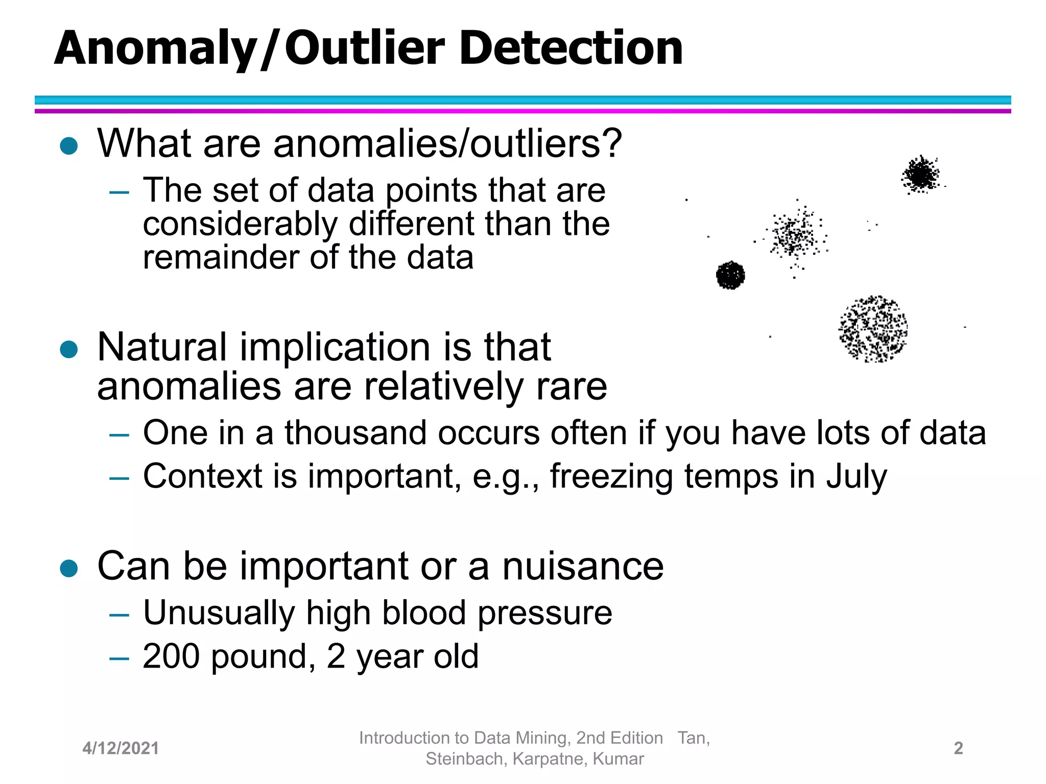
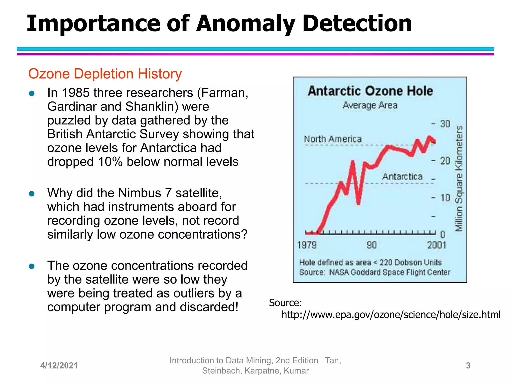
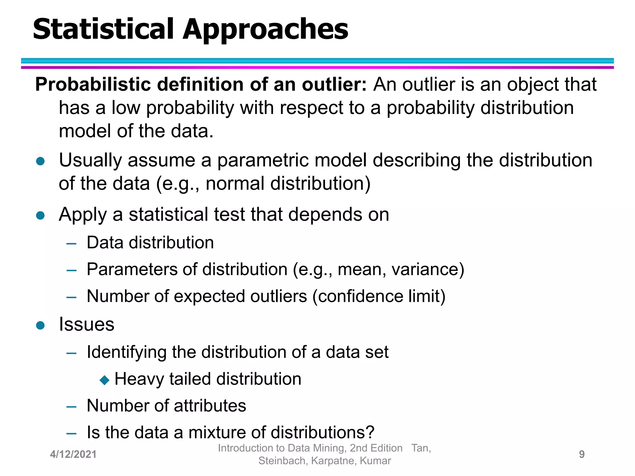
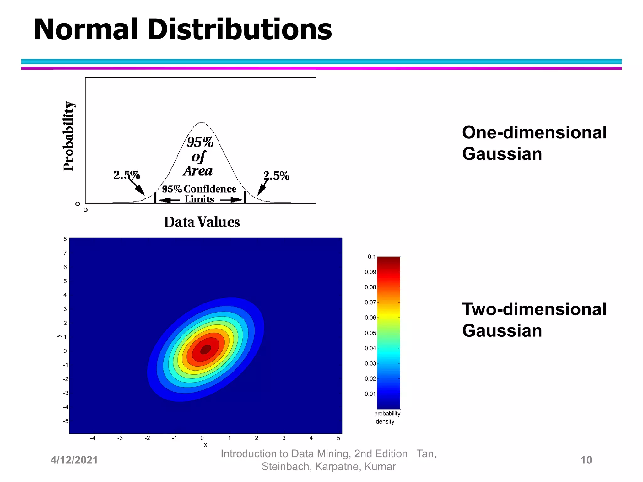
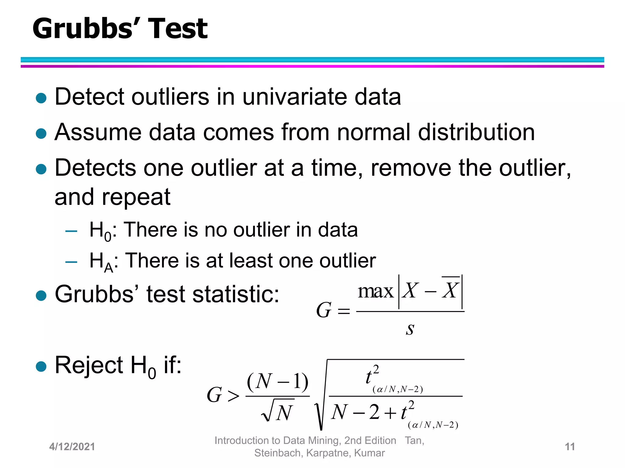
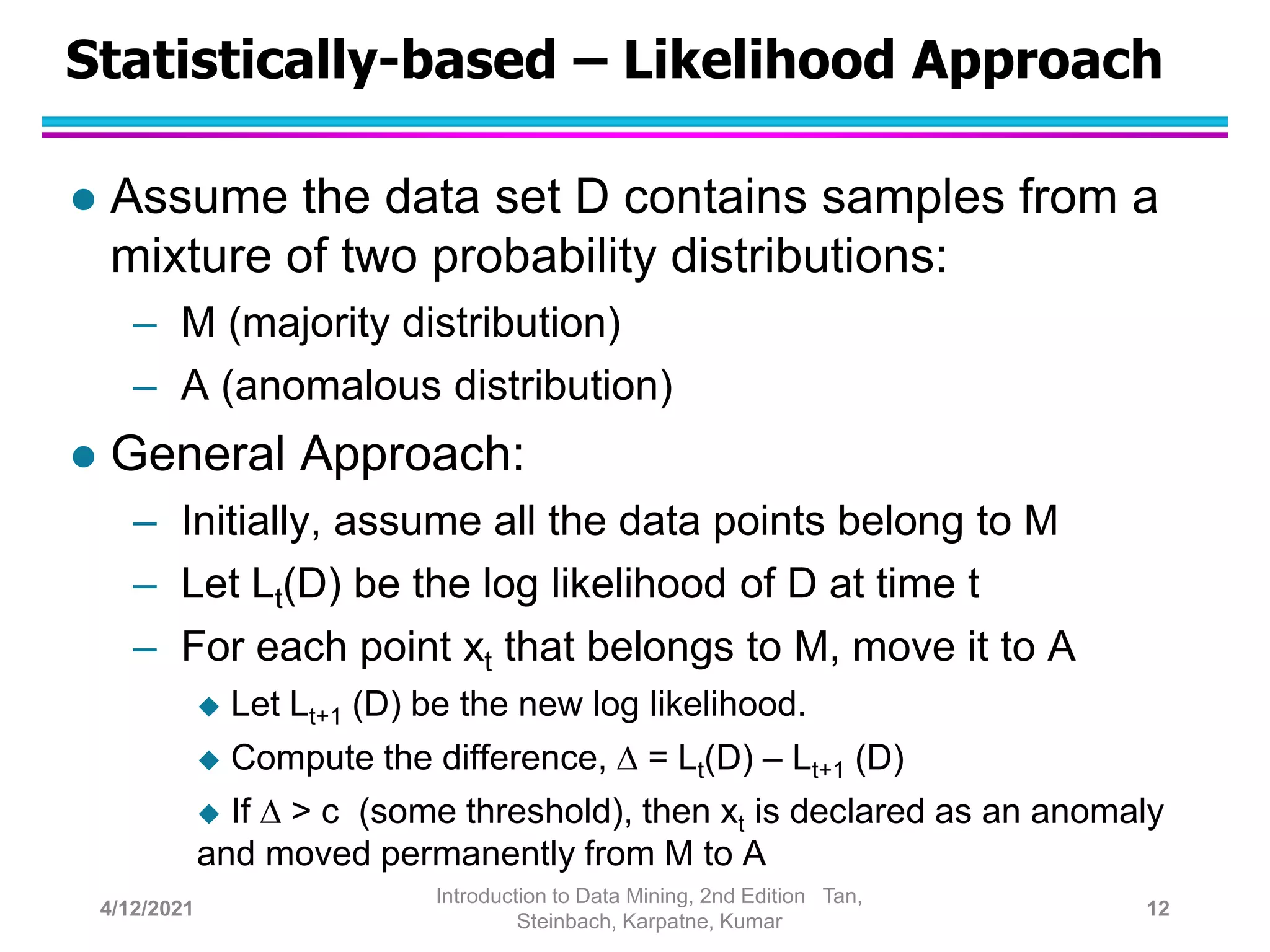
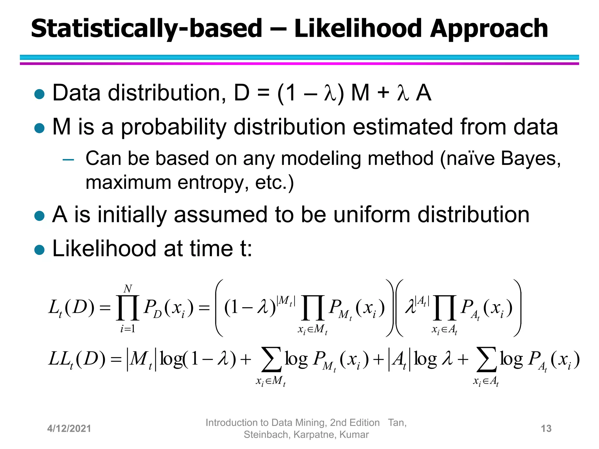
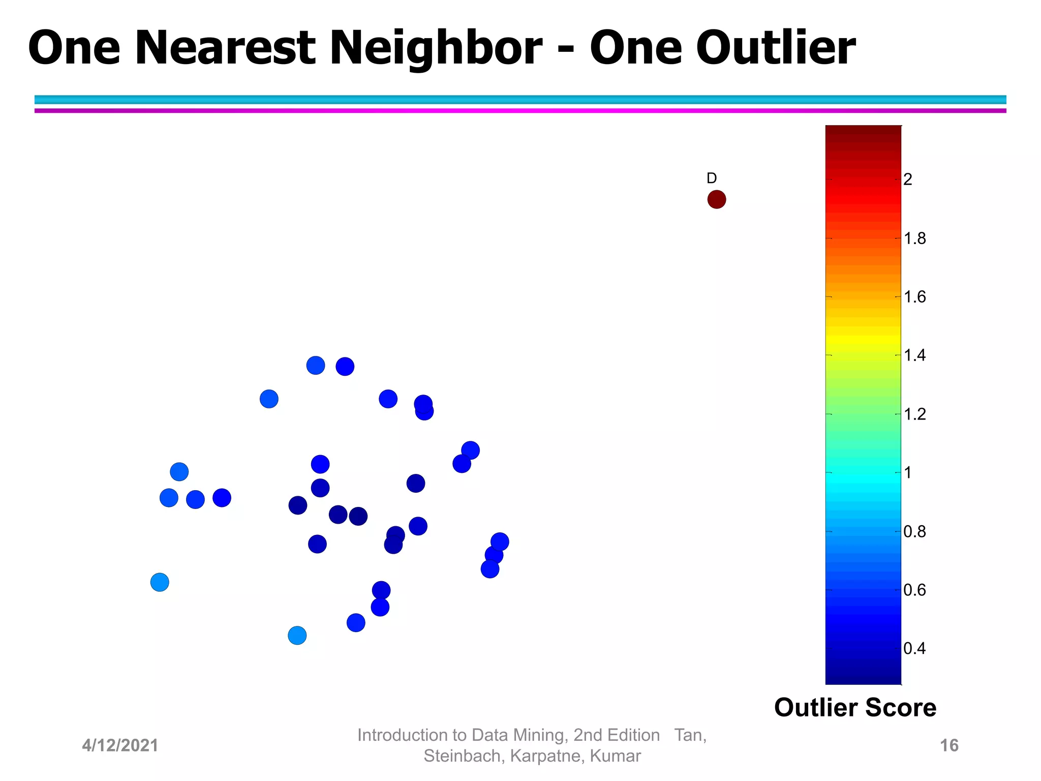
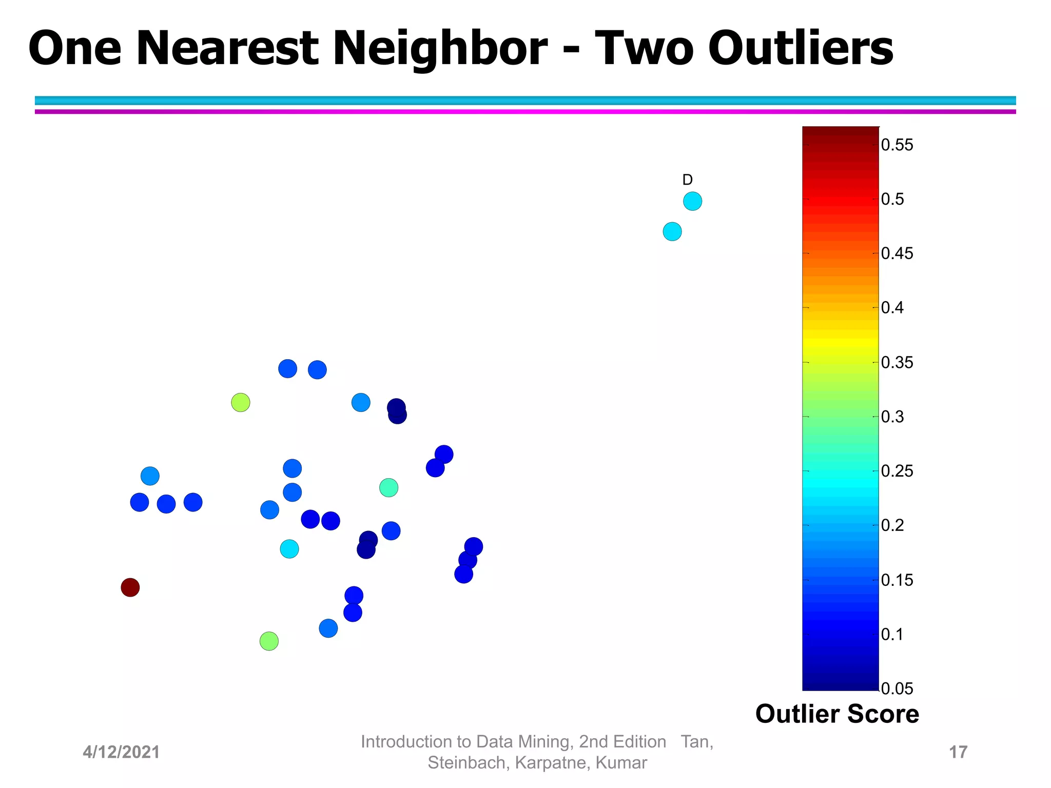
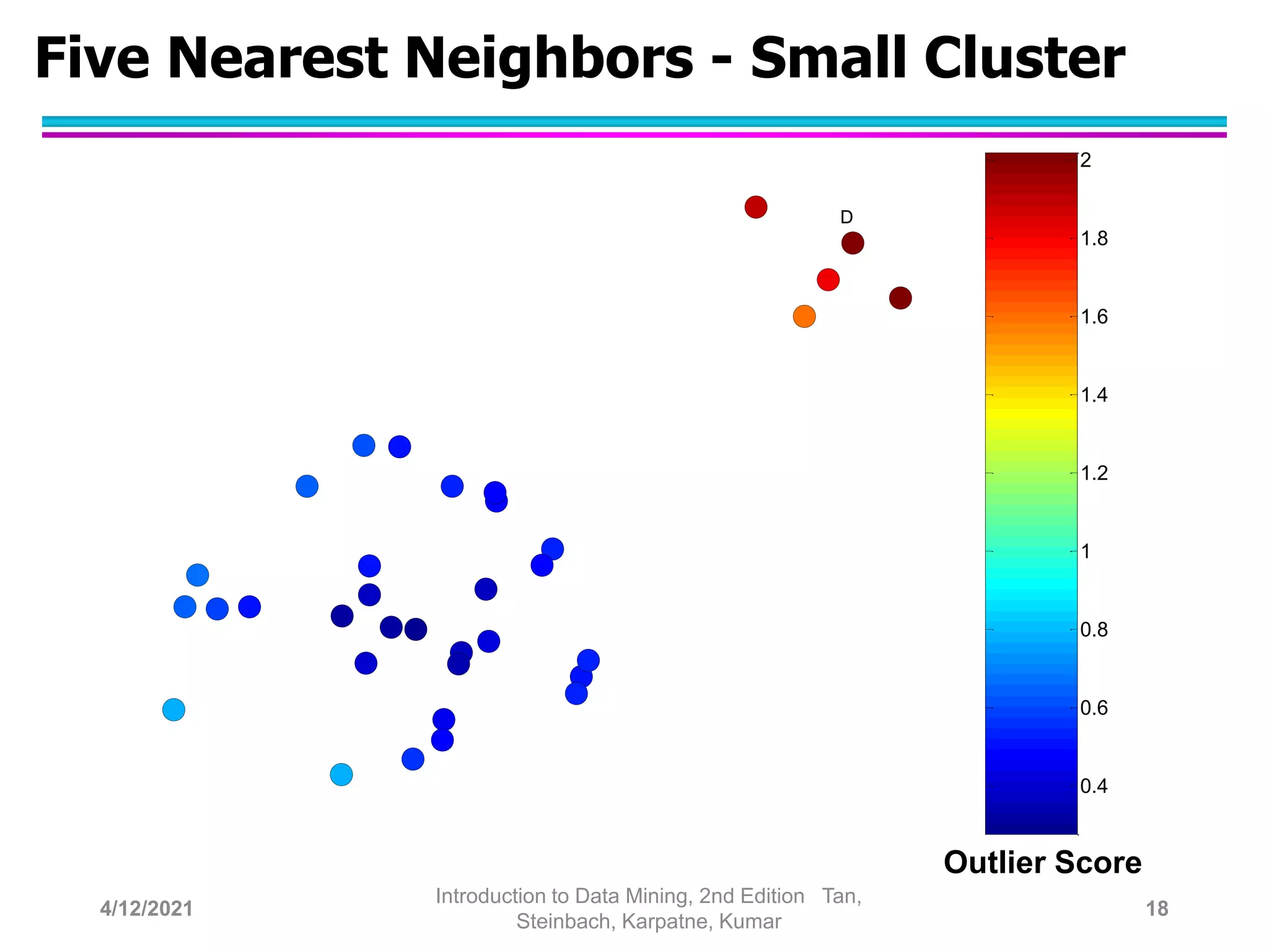
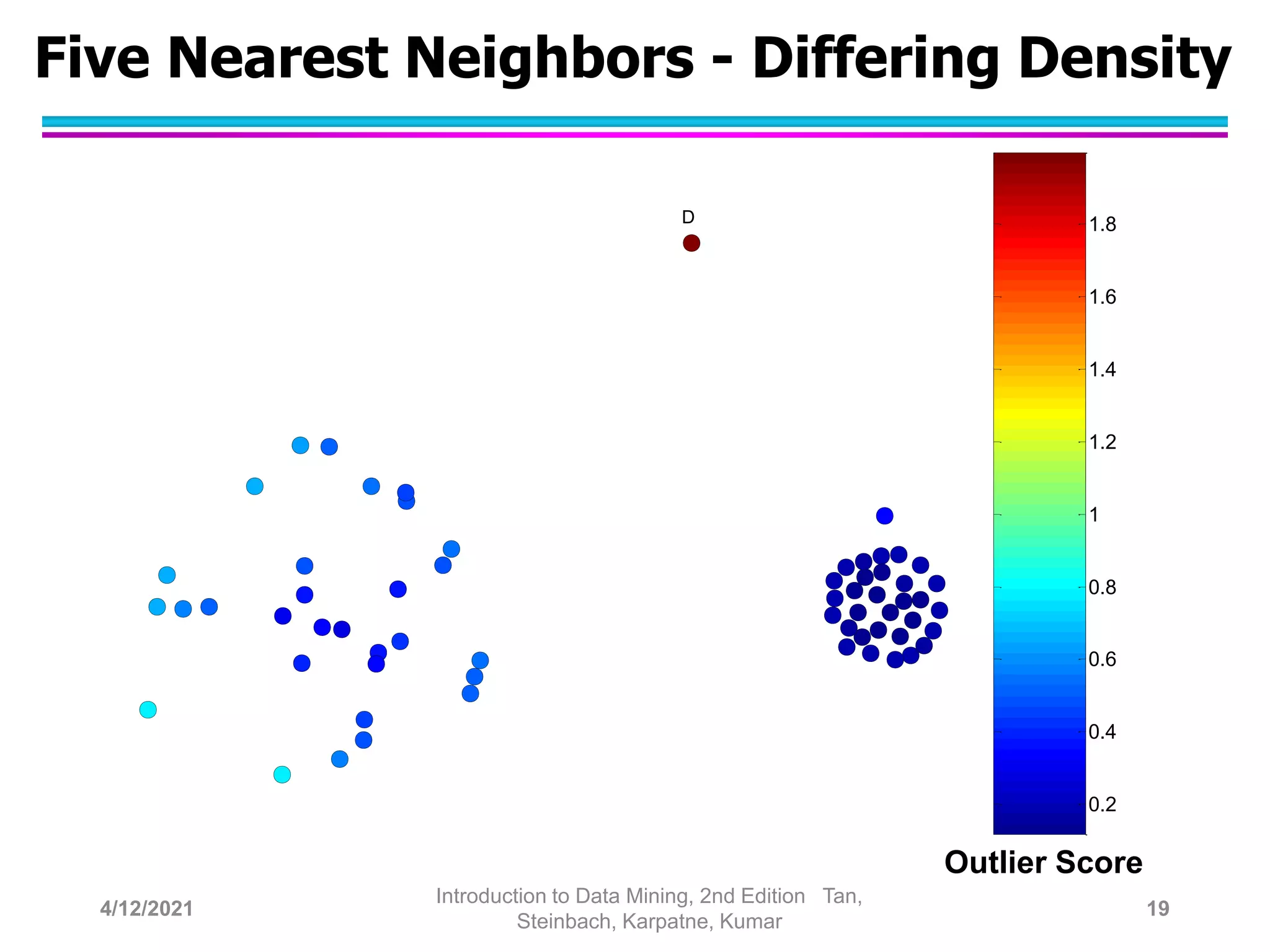
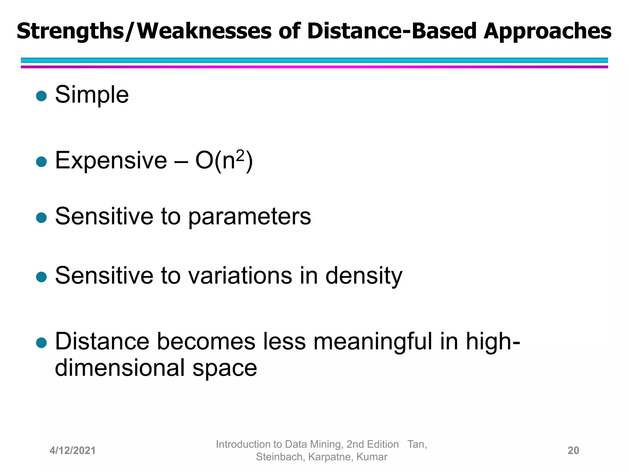
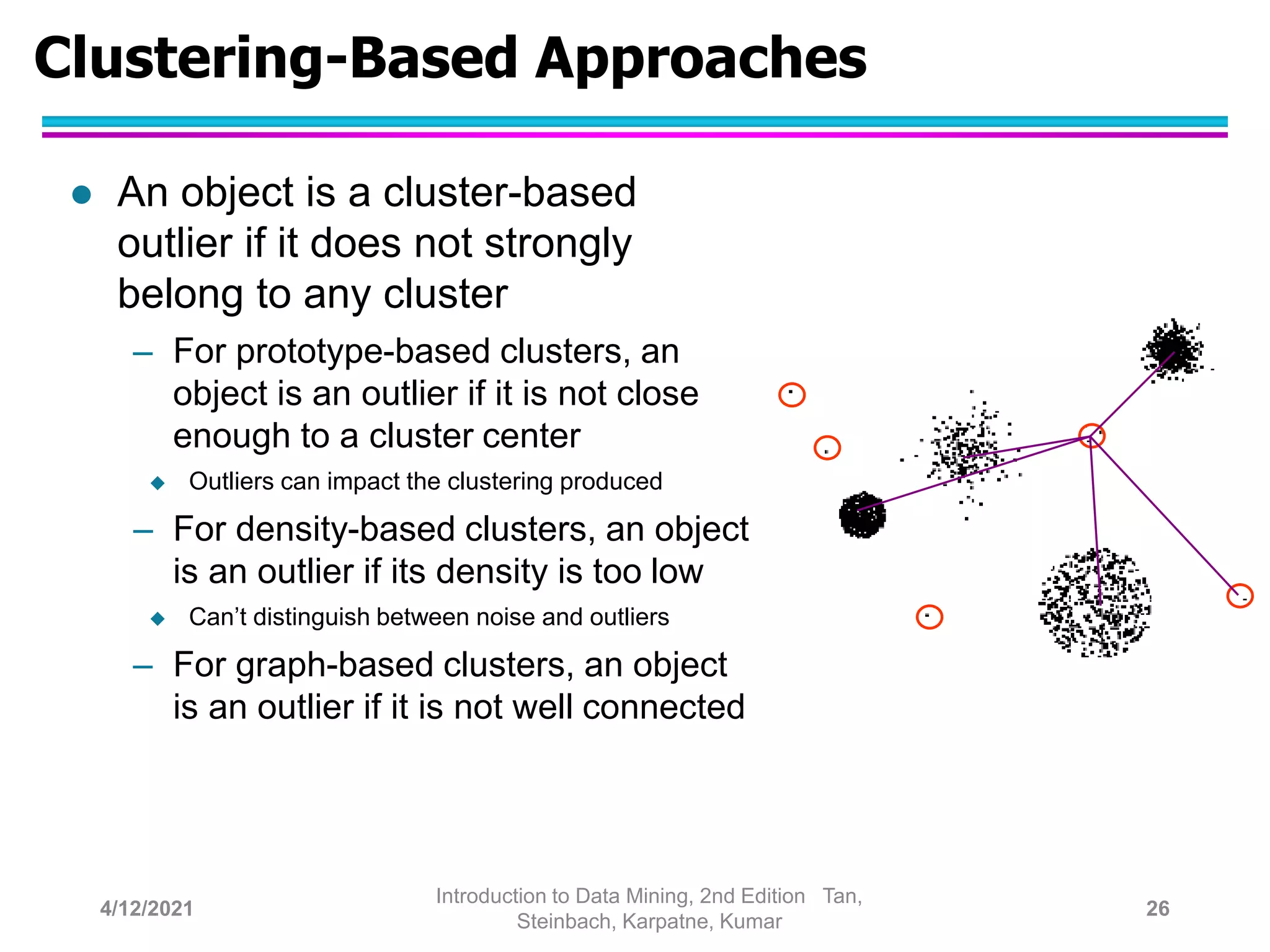
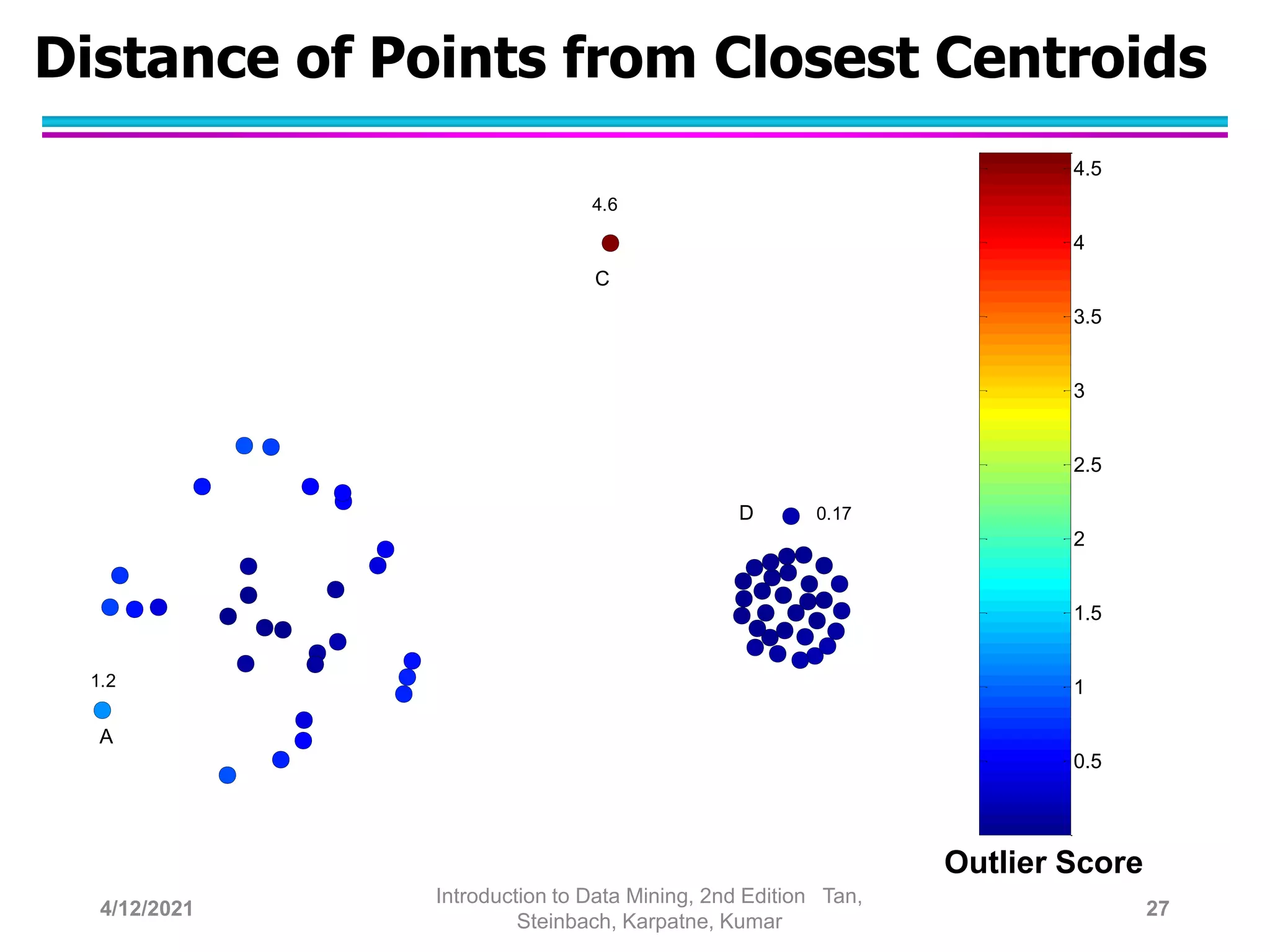
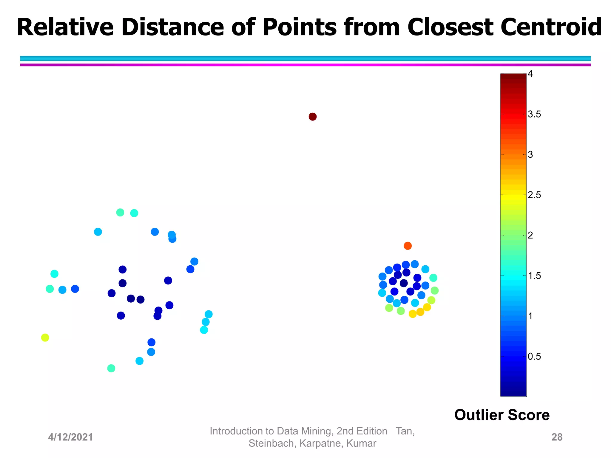
Anomaly Detection
Lecture Notes for Chapter 9
Introduction to Data Mining, 2nd Edition
by
Tan, Steinbach, Karpatne, Kumar
4/12/2021
Introduction to Data Mining, 2nd Edition Tan,
Steinbach, Karpatne, Kumar
1

Anomaly/Outlier Detection
 What are anomalies/outliers?
– The set of data points that are
considerably different than the
remainder of the data
 Natural implication is that
anomalies are relatively rare
– One in a thousand occurs often if you have lots of data
– Context is important, e.g., freezing temps in July
 Can be important or a nuisance
– Unusually high blood pressure
– 200 pound, 2 year old
4/12/2021
2

Importance of Anomaly Detection
Ozone Depletion History
 In 1985 three researchers (Farman,
Gardinar and Shanklin) were
puzzled by data gathered by the
British Antarctic Survey showing that
ozone levels for Antarctica had
dropped 10% below normal levels
 Why did the Nimbus 7 satellite,
which had instruments aboard for
recording ozone levels, not record
similarly low ozone concentrations?
 The ozone concentrations recorded
by the satellite were so low they
were being treated as outliers by a
computer program and discarded! Source:
http://www.epa.gov/ozone/science/hole/size.html
4/12/2021
3

Causes of Anomalies
 Data from different classes
– Measuring the weights of oranges, but a few grapefruit
are mixed in
 Natural variation
– Unusually tall people
 Data errors
– 200 pound 2 year old
4/12/2021
4
https://umn.zoom.us/my/kumar001

Distinction Between Noise and Anomalies
 Noise doesn’t necessarily produce unusual values or
objects
 Noise is not interesting
 Noise and anomalies are related but distinct concepts
4/12/2021
5

Model-based vs Model-free
Model-based Approaches
Model can be parametric or non-parametric
Anomalies are those points that don’t fit well
Anomalies are those points that distort the model
Model-free Approaches
Anomalies are identified directly from the data without
building a model
Often the underlying assumption is that the
most of the points in the data are normal
4/12/2021
6

General Issues: Label vs Score
 Some anomaly detection techniques provide only a
binary categorization
 Other approaches measure the degree to which an
object is an anomaly
– This allows objects to be ranked
– Scores can also have associated meaning (e.g., statistical
significance)
4/12/2021
7

Anomaly Detection Techniques
 Statistical Approaches
 Proximity-based
– Anomalies are points far away from other points
 Clustering-based
– Points far away from cluster centers are outliers
– Small clusters are outliers
 Reconstruction Based
4/12/2021
8

Statistical Approaches
Probabilistic definition of an outlier: An outlier is an object that
has a low probability with respect to a probability distribution
model of the data.
 Usually assume a parametric model describing the distribution
of the data (e.g., normal distribution)
 Apply a statistical test that depends on
– Data distribution
– Parameters of distribution (e.g., mean, variance)
– Number of expected outliers (confidence limit)
 Issues
– Identifying the distribution of a data set
 Heavy tailed distribution
– Number of attributes
– Is the data a mixture of distributions?
4/12/2021
9

Normal Distributions
One-dimensional
Gaussian
Two-dimensional
Gaussian
x
y
-4 -3 -2 -1 0 1 2 3 4 5
-5
-4
-3
-2
-1
0
1
2
3
4
5
6
7
8
probability
density
0.01
0.02
0.03
0.04
0.05
0.06
0.07
0.08
0.09
0.1
4/12/2021
10

Grubbs’ Test
 Detect outliers in univariate data
 Assume data comes from normal distribution
 Detects one outlier at a time, remove the outlier,
and repeat
– H0: There is no outlier in data
– HA: There is at least one outlier
 Grubbs’ test statistic:
 Reject H0 if:
s
X
X
G


max
2
2
)
2
,
/
(
)
2
,
/
(
2
)
1
(






N
N
N
N
t
N
t
N
N
G


4/12/2021
11

Statistically-based – Likelihood Approach
 Assume the data set D contains samples from a
mixture of two probability distributions:
– M (majority distribution)
– A (anomalous distribution)
 General Approach:
– Initially, assume all the data points belong to M
– Let Lt(D) be the log likelihood of D at time t
– For each point xt that belongs to M, move it to A
 Let Lt+1 (D) be the new log likelihood.
 Compute the difference,  = Lt(D) – Lt+1 (D)
 If  > c (some threshold), then xt is declared as an anomaly
and moved permanently from M to A
4/12/2021
12

Statistically-based – Likelihood Approach
 Data distribution, D = (1 – ) M +  A
 M is a probability distribution estimated from data
– Can be based on any modeling method (naïve Bayes,
maximum entropy, etc.)
 A is initially assumed to be uniform distribution
 Likelihood at time t:


































t
i
t
t
i
t
t
i
t
t
t
i
t
t
A
x
i
A
t
M
x
i
M
t
t
A
x
i
A
A
M
x
i
M
M
N
i
i
D
t
x
P
A
x
P
M
D
LL
x
P
x
P
x
P
D
L
)
(
log
log
)
(
log
)
1
log(
)
(
)
(
)
(
)
1
(
)
(
)
( |
|
|
|
1




4/12/2021
13

Strengths/Weaknesses of Statistical Approaches
 Firm mathematical foundation
 Can be very efficient
 Good results if distribution is known
 In many cases, data distribution may not be known
 For high dimensional data, it may be difficult to estimate
the true distribution
 Anomalies can distort the parameters of the distribution
4/12/2021
14

Distance-Based Approaches
 The outlier score of an object is the distance to
its kth nearest neighbor
4/12/2021
15

One Nearest Neighbor - One Outlier
D
0.4
0.6
0.8
1
1.2
1.4
1.6
1.8
2
Outlier Score
4/12/2021
16

One Nearest Neighbor - Two Outliers
D
0.05
0.1
0.15
0.2
0.25
0.3
0.35
0.4
0.45
0.5
0.55
Outlier Score
4/12/2021
17

Five Nearest Neighbors - Small Cluster
D
0.4
0.6
0.8
1
1.2
1.4
1.6
1.8
2
Outlier Score
4/12/2021
18

Five Nearest Neighbors - Differing Density
D
0.2
0.4
0.6
0.8
1
1.2
1.4
1.6
1.8
Outlier Score
4/12/2021
19

Strengths/Weaknesses of Distance-Based Approaches
 Simple
 Expensive – O(n2)
 Sensitive to parameters
 Sensitive to variations in density
 Distance becomes less meaningful in high-
dimensional space
4/12/2021
20

Density-Based Approaches
 Density-based Outlier: The outlier score of an
object is the inverse of the density around the
object.
– Can be defined in terms of the k nearest neighbors
– One definition: Inverse of distance to kth neighbor
– Another definition: Inverse of the average distance to k
neighbors
– DBSCAN definition
 If there are regions of different density, this
approach can have problems
4/12/2021
21

Relative Density
 Consider the density of a point relative to that of
its k nearest neighbors
 Let 𝑦1, … , 𝑦𝑘 be the 𝑘 nearest neighbors of 𝒙
𝑑𝑒𝑛𝑠𝑖𝑡𝑦 𝒙, 𝑘 =
1
𝑑𝑖𝑠𝑡 𝒙, 𝑘
=
1
𝑑𝑖𝑠𝑡(𝒙, 𝒚𝑘)
𝑟𝑒𝑙𝑎𝑡𝑖𝑣𝑒 𝑑𝑒𝑛𝑠𝑖𝑡𝑦 𝒙, 𝑘 = 𝑖=1
𝑘
𝑑𝑒𝑛𝑠𝑖𝑡𝑦(𝒚𝑖,𝑘)/𝑘
𝑑𝑒𝑛𝑠𝑖𝑡𝑦(𝒙,𝑘)
=
𝑑𝑖𝑠𝑡(𝒙,𝑘)
𝑖=1
𝑘
𝑑𝑖𝑠𝑡(𝒚𝑖,𝑘)/𝑘
=
𝑑𝑖𝑠𝑡(𝒙,𝒚)
𝑖=1
𝑘
𝑑𝑖𝑠𝑡(𝒚𝑖,𝑘)/𝑘
 Can use average distance instead
4/12/2021
22

Relative Density Outlier Scores
Outlier Score
1
2
3
4
5
6
6.85
1.33
1.40
A
C
D
4/12/2021
23

Relative Density-based: LOF approach
 For each point, compute the density of its local neighborhood
 Compute local outlier factor (LOF) of a sample p as the average of
the ratios of the density of sample p and the density of its nearest
neighbors
 Outliers are points with largest LOF value
p2
 p1

In the NN approach, p2 is
not considered as outlier,
while LOF approach find
both p1 and p2 as outliers
4/12/2021
24

Strengths/Weaknesses of Density-Based Approaches
 Simple
 Expensive – O(n2)
 Sensitive to parameters
 Density becomes less meaningful in high-
dimensional space
4/12/2021
25

Clustering-Based Approaches
 An object is a cluster-based
outlier if it does not strongly
belong to any cluster
– For prototype-based clusters, an
object is an outlier if it is not close
enough to a cluster center
 Outliers can impact the clustering produced
– For density-based clusters, an object
is an outlier if its density is too low
 Can’t distinguish between noise and outliers
– For graph-based clusters, an object
is an outlier if it is not well connected
4/12/2021
26

Distance of Points from Closest Centroids
Outlier Score
0.5
1
1.5
2
2.5
3
3.5
4
4.5
D
C
A
1.2
0.17
4.6
4/12/2021
27

Relative Distance of Points from Closest Centroid
Outlier Score
0.5
1
1.5
2
2.5
3
3.5
4
4/12/2021
28

Strengths/Weaknesses of Clustering-Based Approaches
 Simple
 Many clustering techniques can be used
 Can be difficult to decide on a clustering
technique
 Can be difficult to decide on number of clusters
 Outliers can distort the clusters
4/12/2021
29

Reconstruction-Based Approaches
 Based on assumptions there are patterns in the
distribution of the normal class that can be
captured using lower-dimensional
representations
 Reduce data to lower dimensional data
– E.g. Use Principal Components Analysis (PCA) or
Auto-encoders
 Measure the reconstruction error for each object
– The difference between original and reduced
dimensionality version
4/12/2021
30

Reconstruction Error
 Let 𝐱 be the original data object
 Find the representation of the object in a lower
dimensional space
 Project the object back to the original space
 Call this object 𝐱
Reconstruction Error(x)= x − x
 Objects with large reconstruction errors are
anomalies
4/12/2021
31

Reconstruction of two-dimensional data
4/12/2021
32

Basic Architecture of an Autoencoder
 An autoencoder is a multi-layer neural network
 The number of input and output neurons is equal
to the number of original attributes.
4/12/2021
Introduction to Data Mining, 2nd Edition
Tan, Steinbach, Karpatne, Kumar
33

Strengths and Weaknesses
 Does not require assumptions about distribution
of normal class
 Can use many dimensionality reduction
approaches
 The reconstruction error is computed in the
original space
– This can be a problem if dimensionality is high
4/12/2021
34

One Class SVM
 Uses an SVM approach to classify normal objects
 Uses the given data to construct such a model
 This data may contain outliers
 But the data does not contain class labels
 How to build a classifier given one class?
4/12/2021
35

How Does One-Class SVM Work?
 Uses the “origin” trick
 Use a Gaussian kernel
– Every point mapped to a unit hypersphere
– Every point in the same orthant (quadrant)
 Aim to maximize the distance of the separating
plane from the origin
4/12/2021
36

Two-dimensional One Class SVM
4/12/2021
37

Equations for One-Class SVM
 Equation of hyperplane
 𝜙 is the mapping to high dimensional space
 Weight vector is
 ν is fraction of outliers
 Optimization condition is the following
4/12/2021
38

Finding Outliers with a One-Class SVM
 Decision boundary with 𝜈 = 0.1
4/12/2021
39

Finding Outliers with a One-Class SVM
 Decision boundary with 𝜈 = 0.05 and 𝜈 = 0.2
4/12/2021
40

 Strong theoretical foundation
 Choice of ν is difficult
 Computationally expensive
4/12/2021
41

Information Theoretic Approaches
 Key idea is to measure how much information
decreases when you delete an observation
 Anomalies should show higher gain
 Normal points should have less gain
4/12/2021
42

Information Theoretic Example
 Survey of height and weight for 100 participants
 Eliminating last group give a gain of
2.08 − 1.89 = 0.19
4/12/2021
43

 Solid theoretical foundation
 Theoretically applicable to all kinds of data
 Difficult and computationally expensive to
implement in practice
4/12/2021
44

Evaluation of Anomaly Detection
 If class labels are present, then use standard
evaluation approaches for rare class such as
precision, recall, or false positive rate
– FPR is also know as false alarm rate
 For unsupervised anomaly detection use
measures provided by the anomaly method
– E.g. reconstruction error or gain
 Can also look at histograms of anomaly scores.
4/12/2021
45

Distribution of Anomaly Scores
 Anomaly scores should show a tail
4/12/2021
46

chap9_anomaly_detection.pptx

More Related Content

Similar to chap9_anomaly_detection.pptx

Recently uploaded

chap9_anomaly_detection.pptx