Chap10 Anomaly Detection

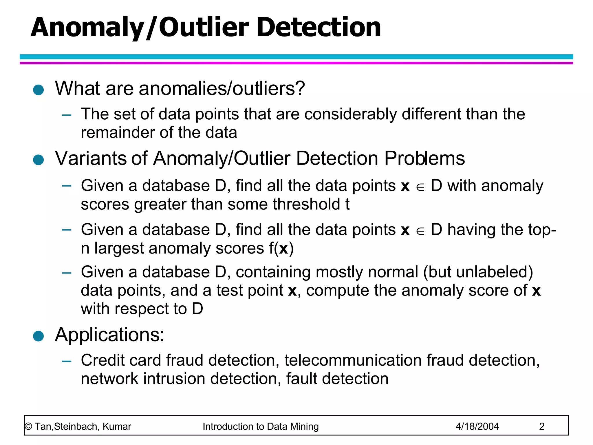
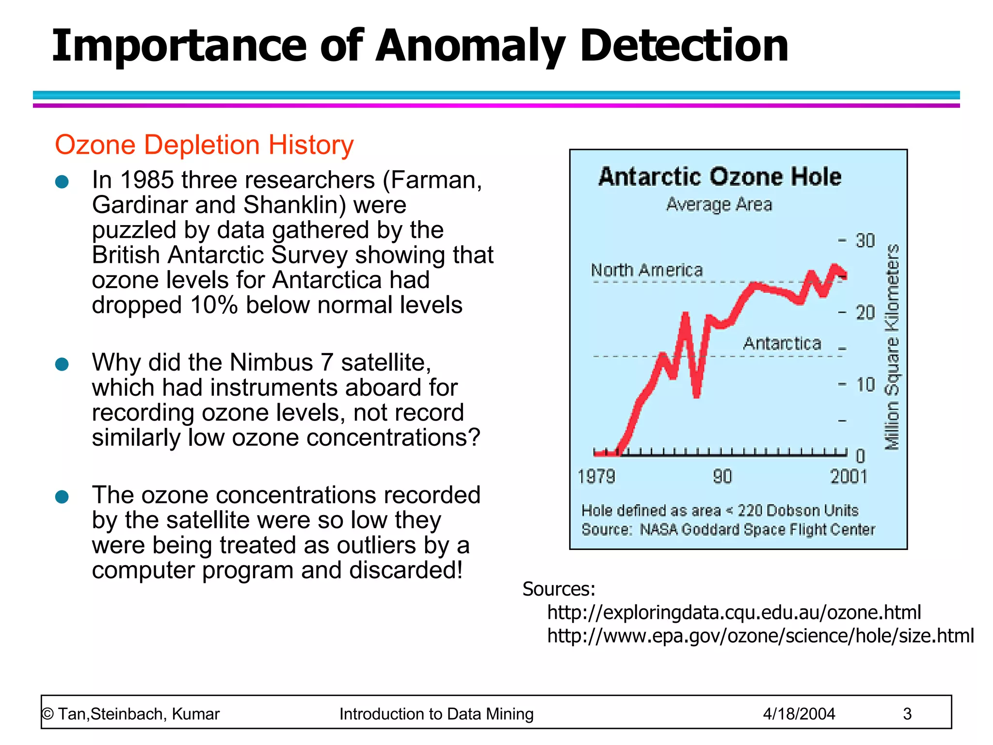
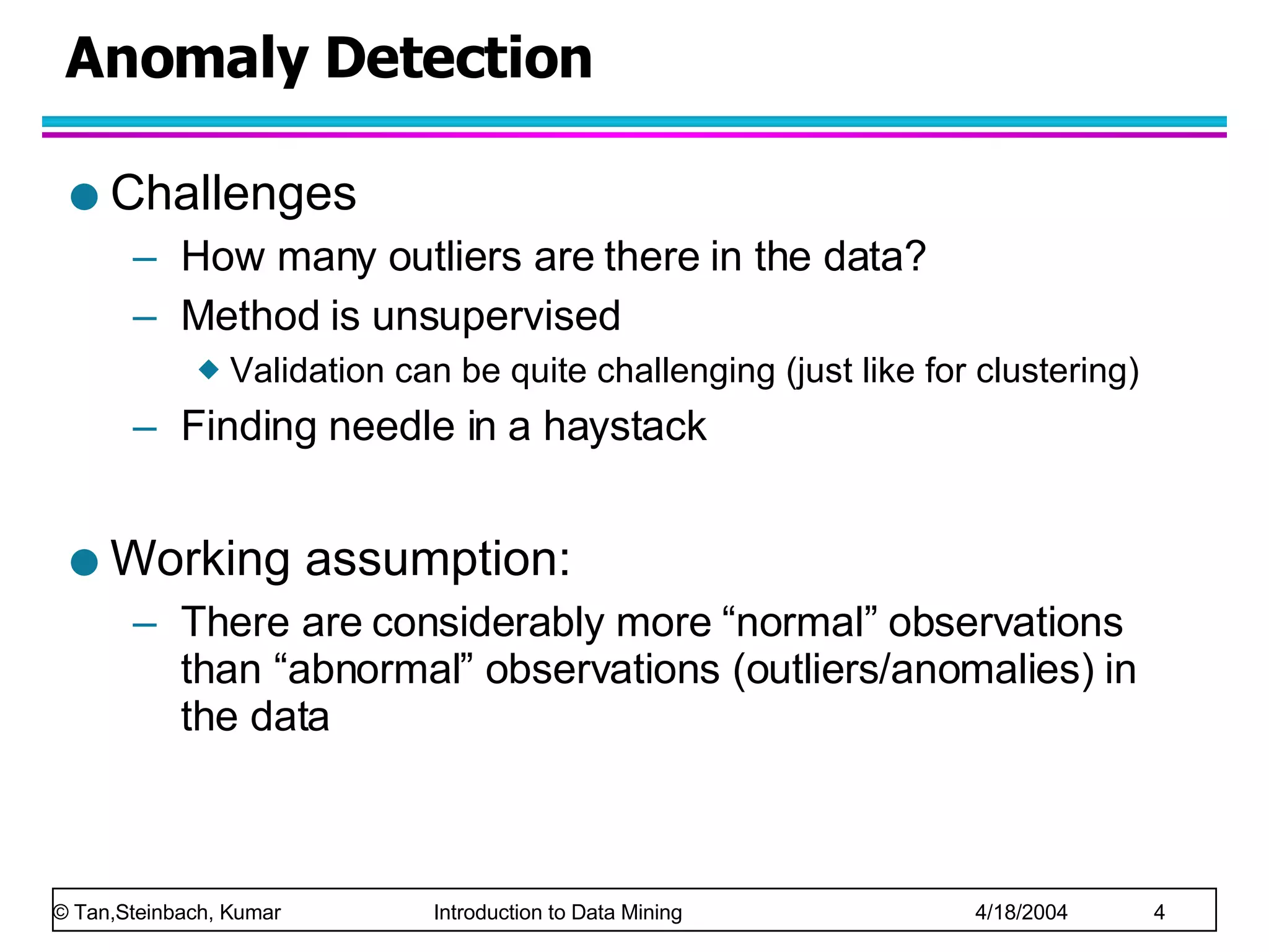
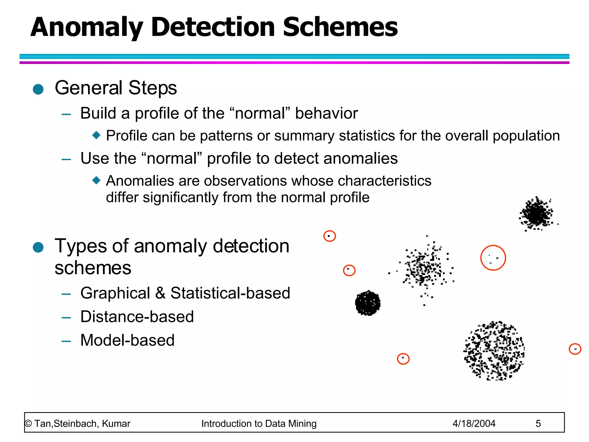
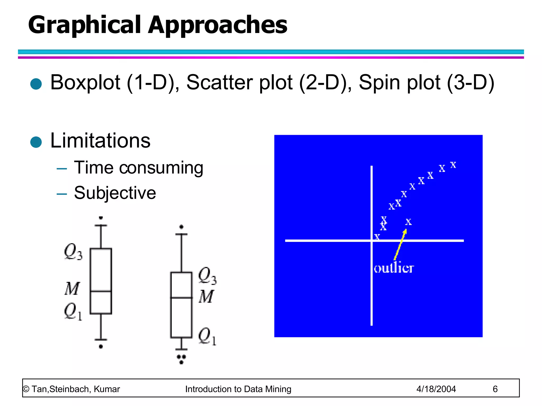
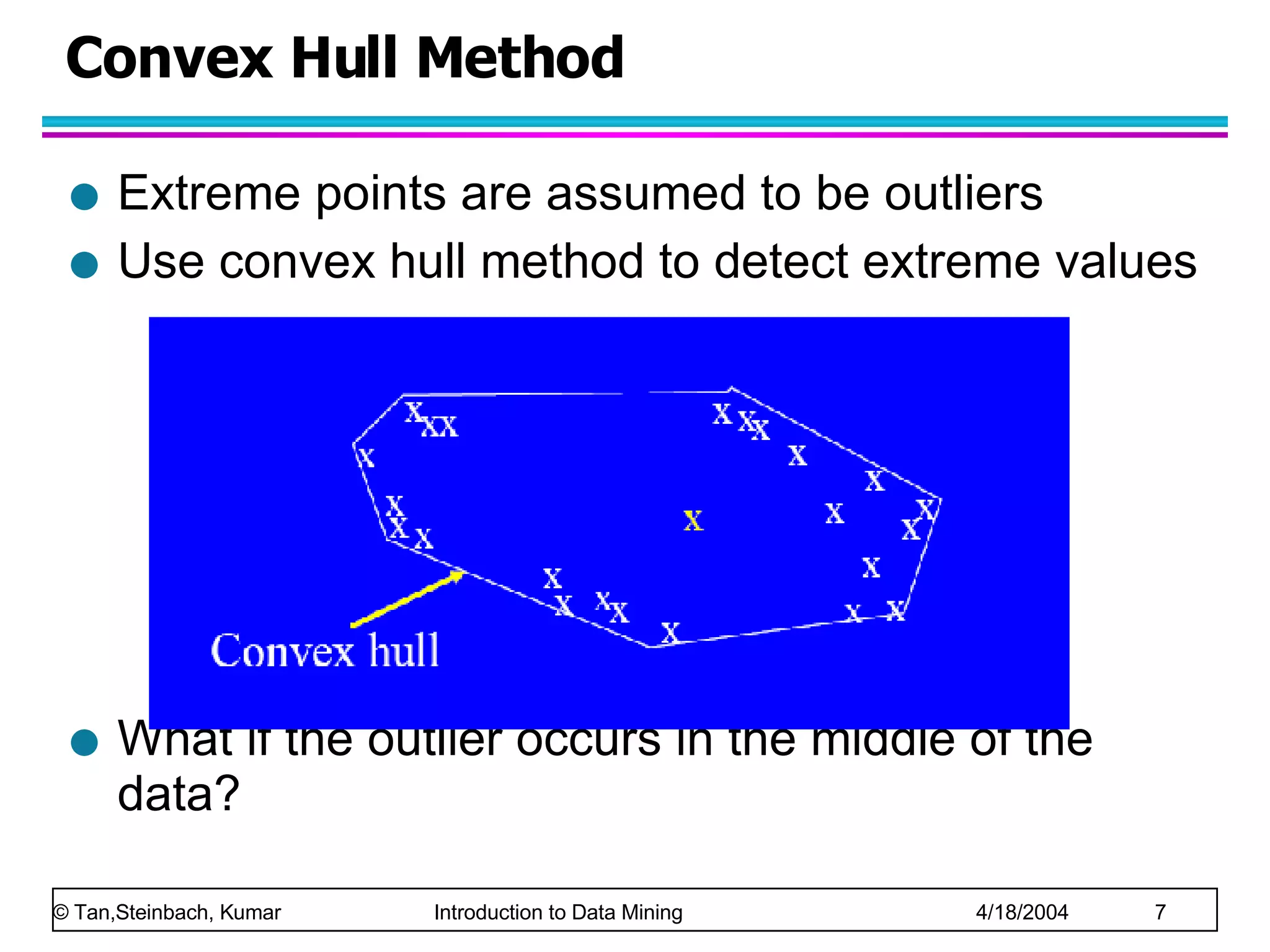
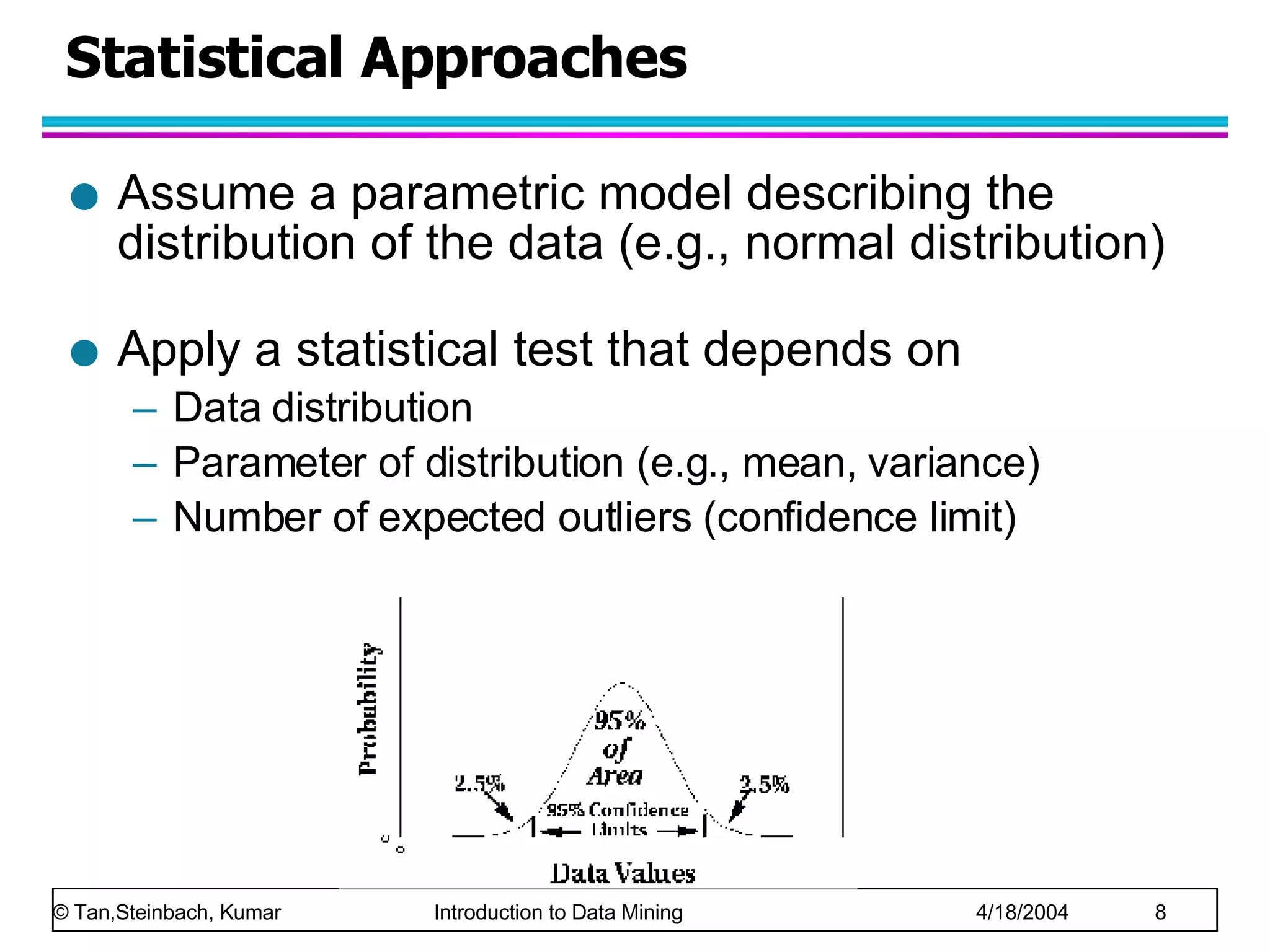
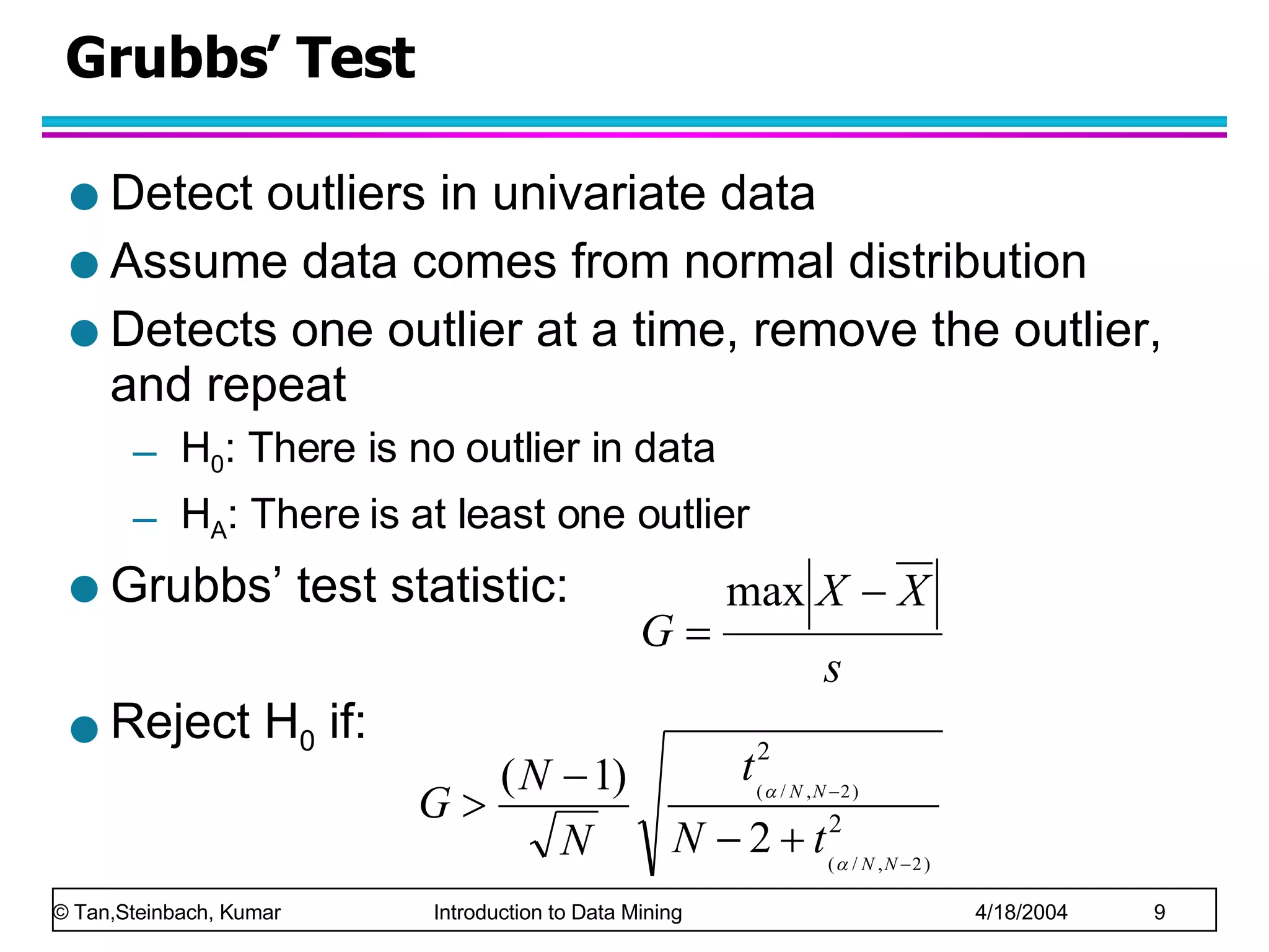
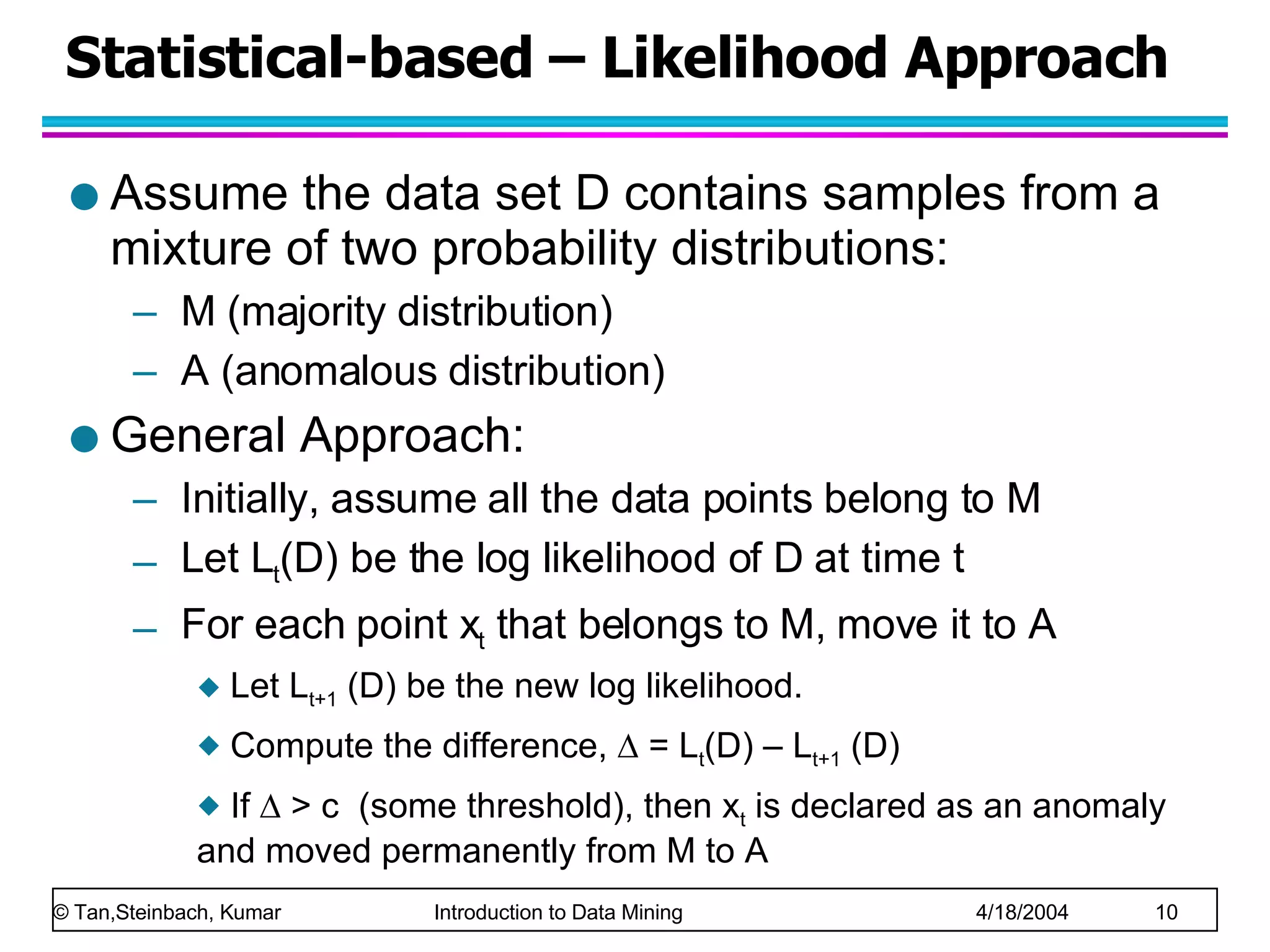
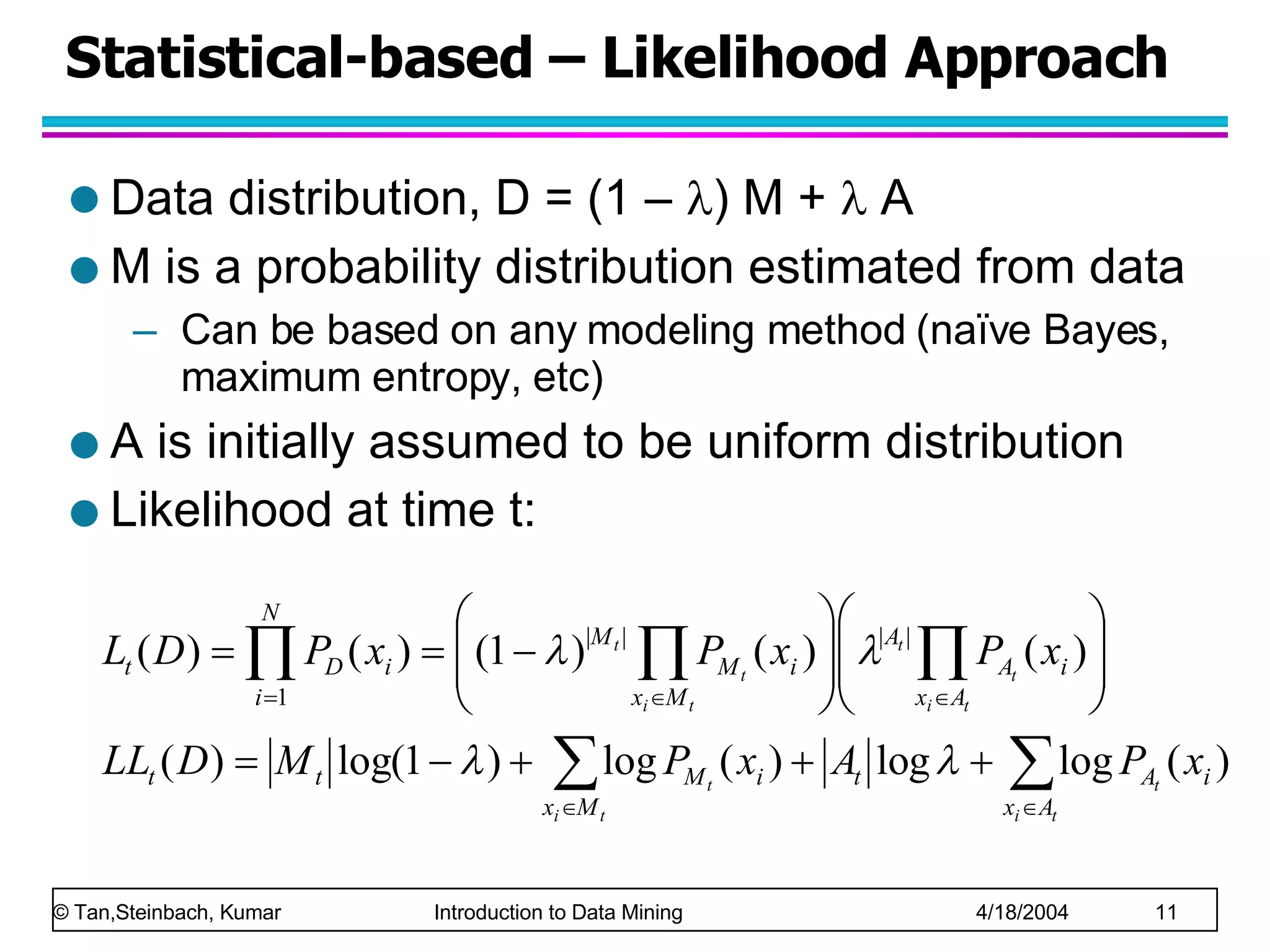
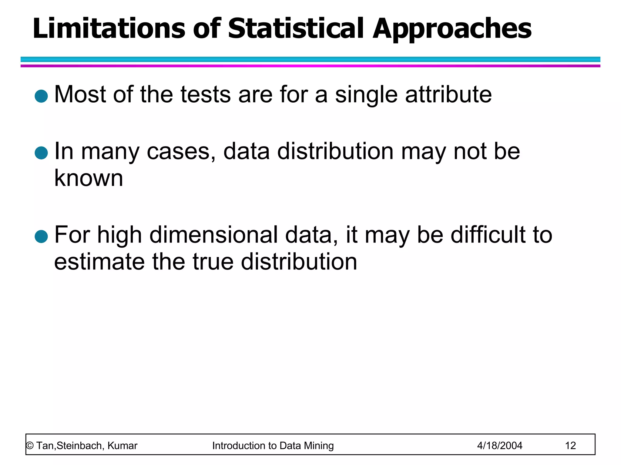
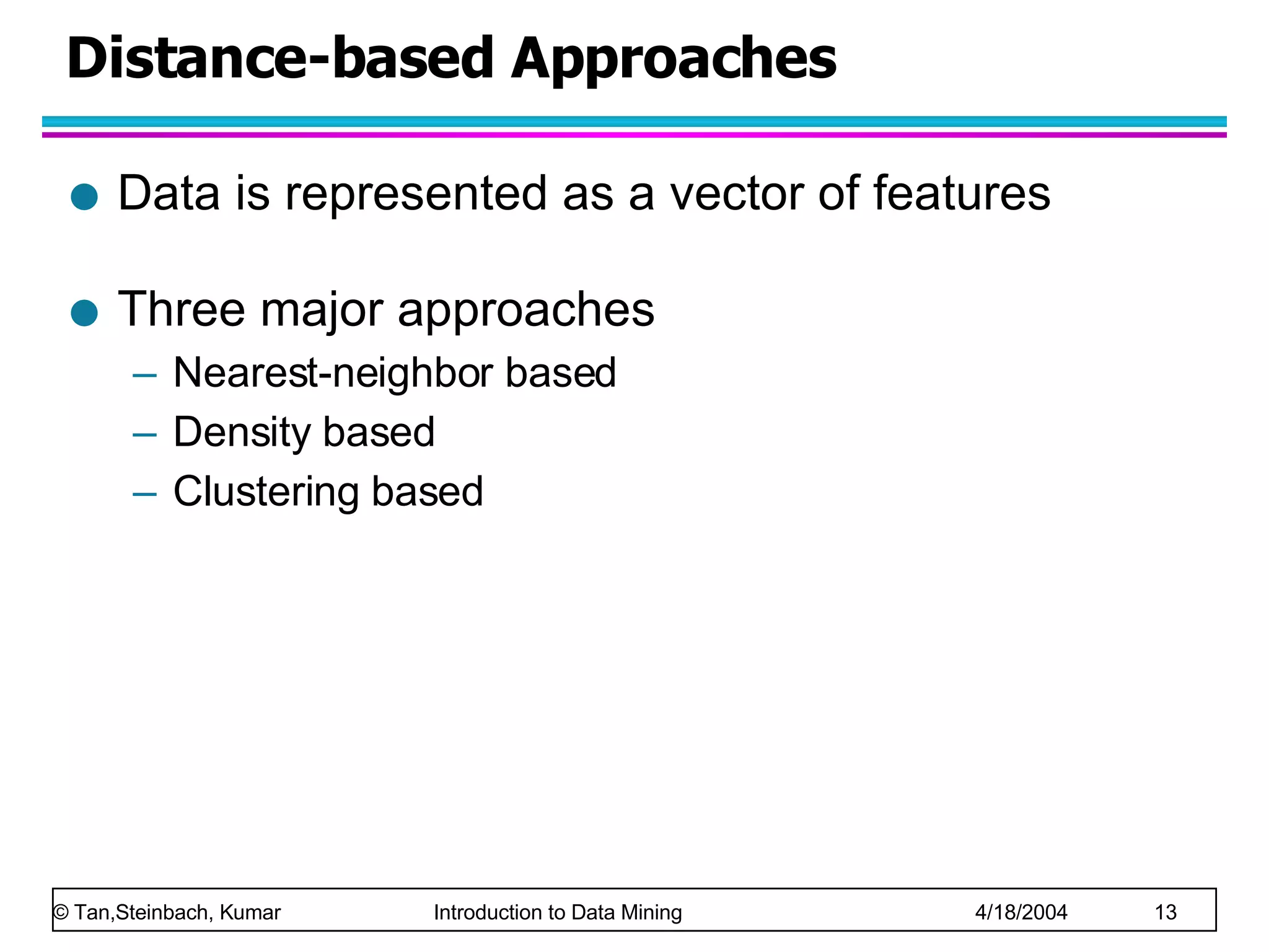
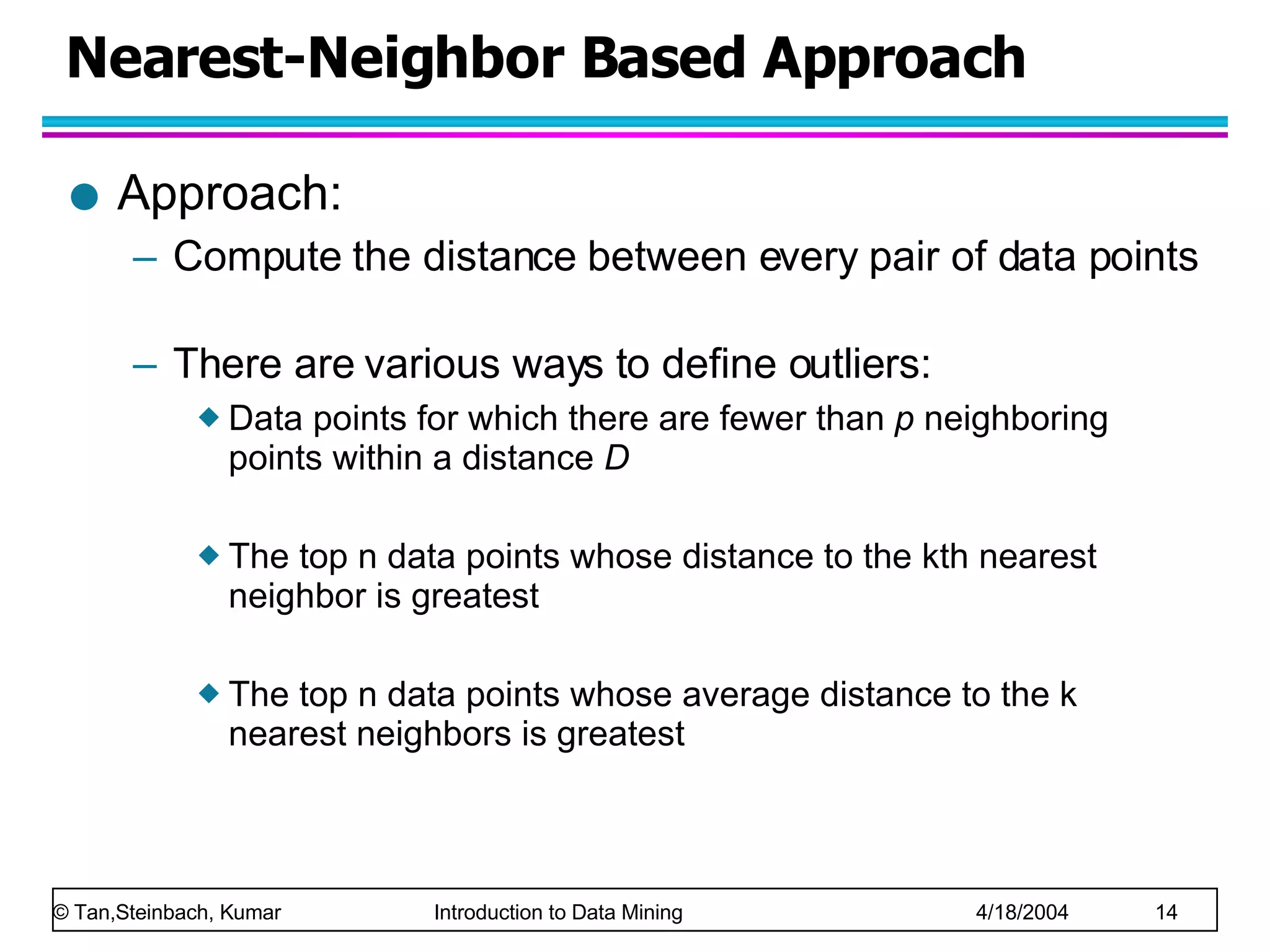
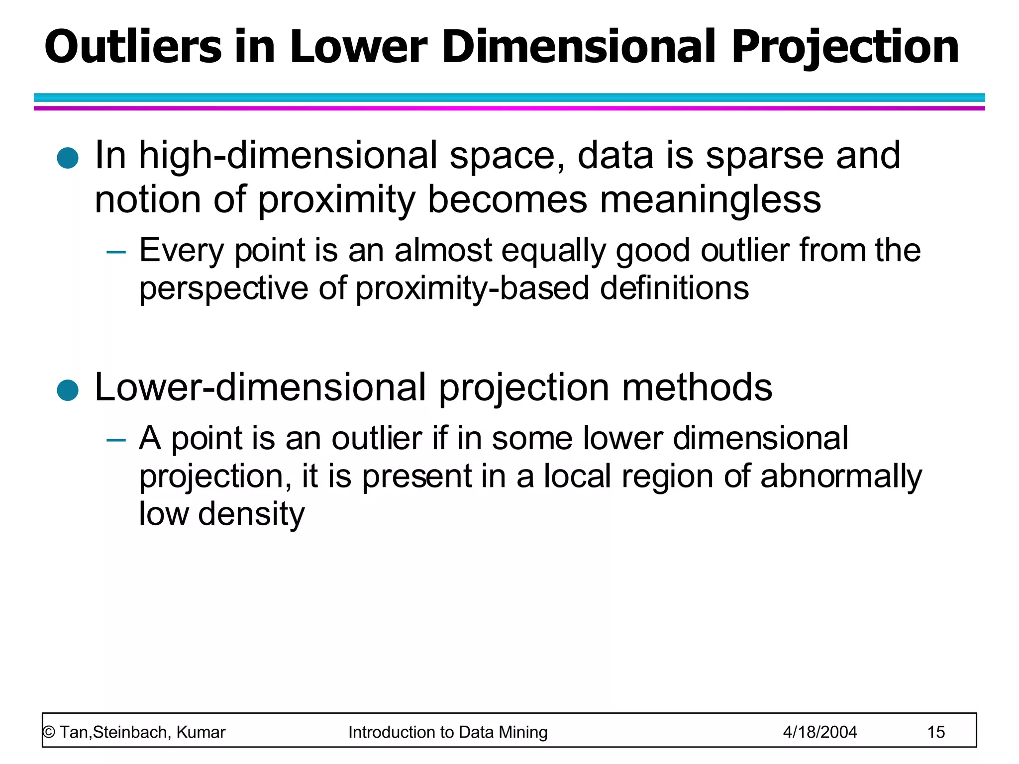
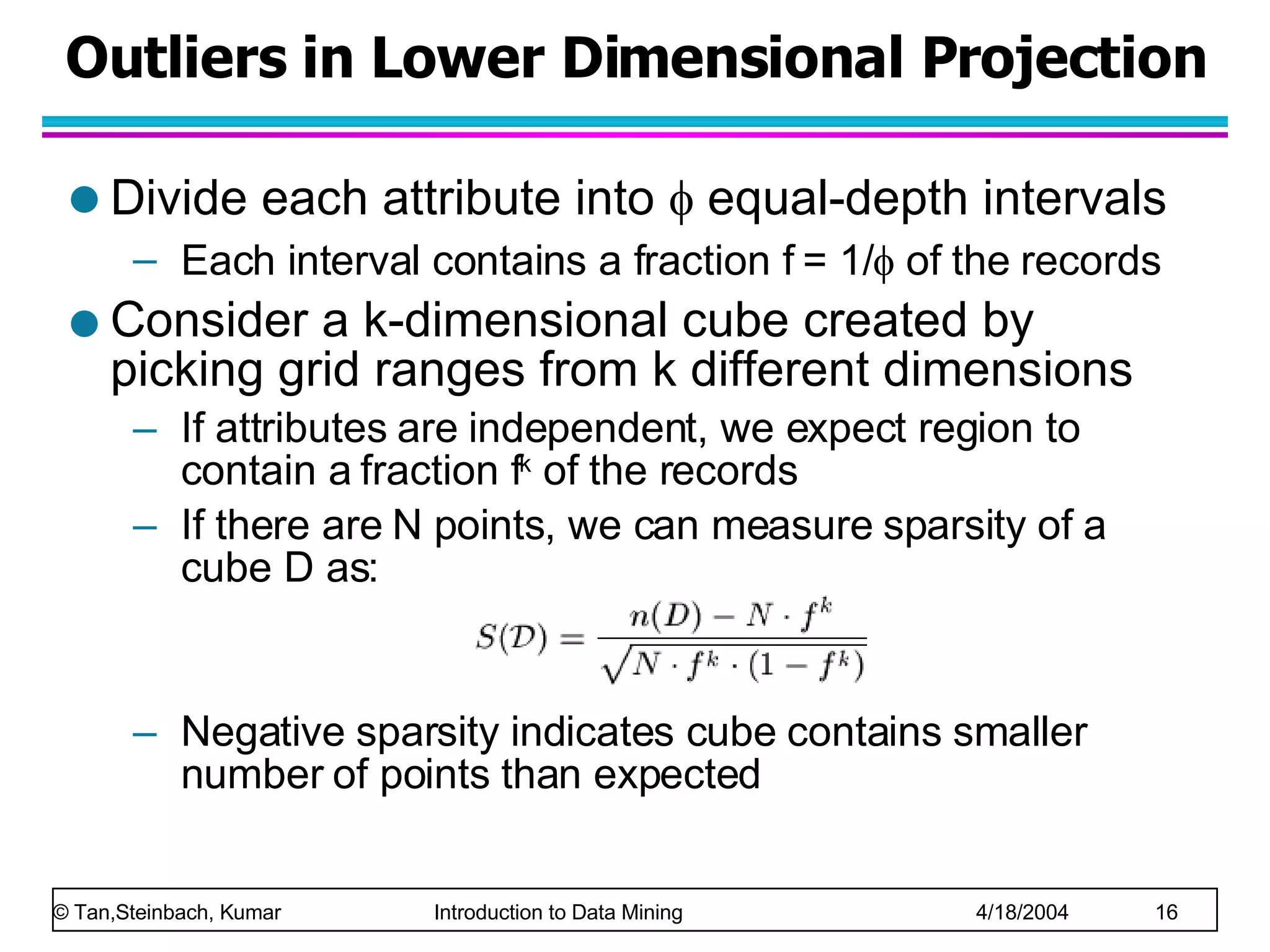
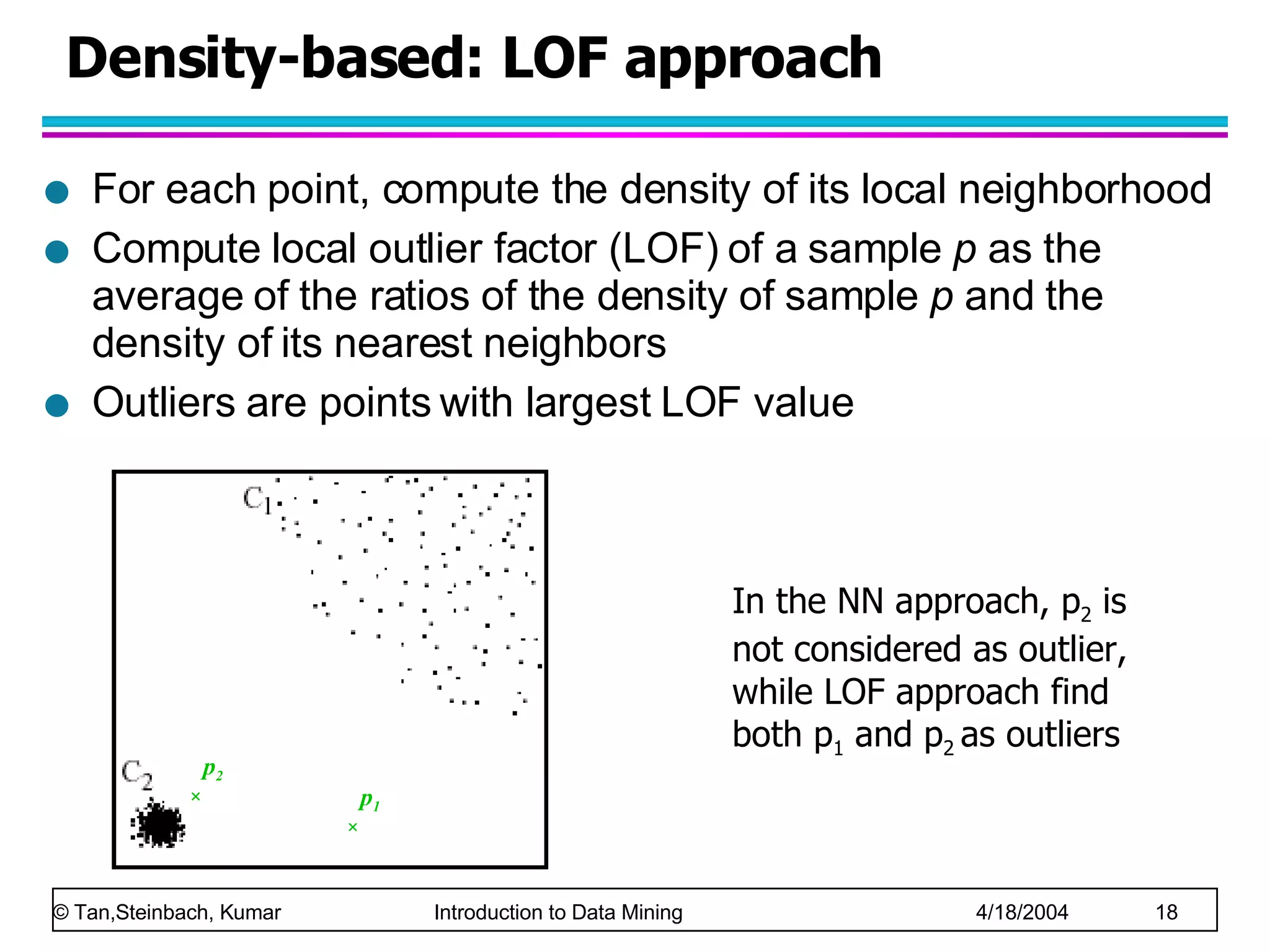
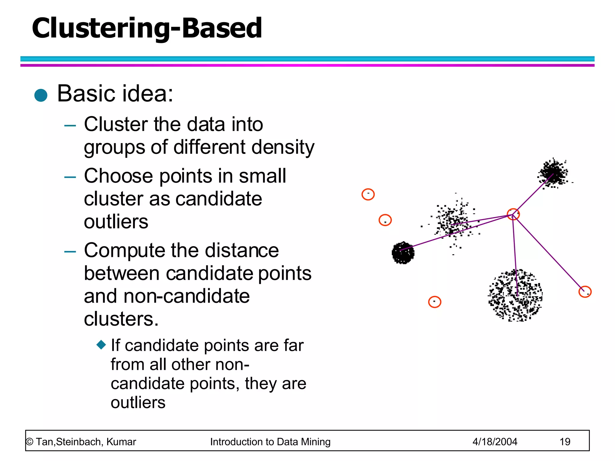
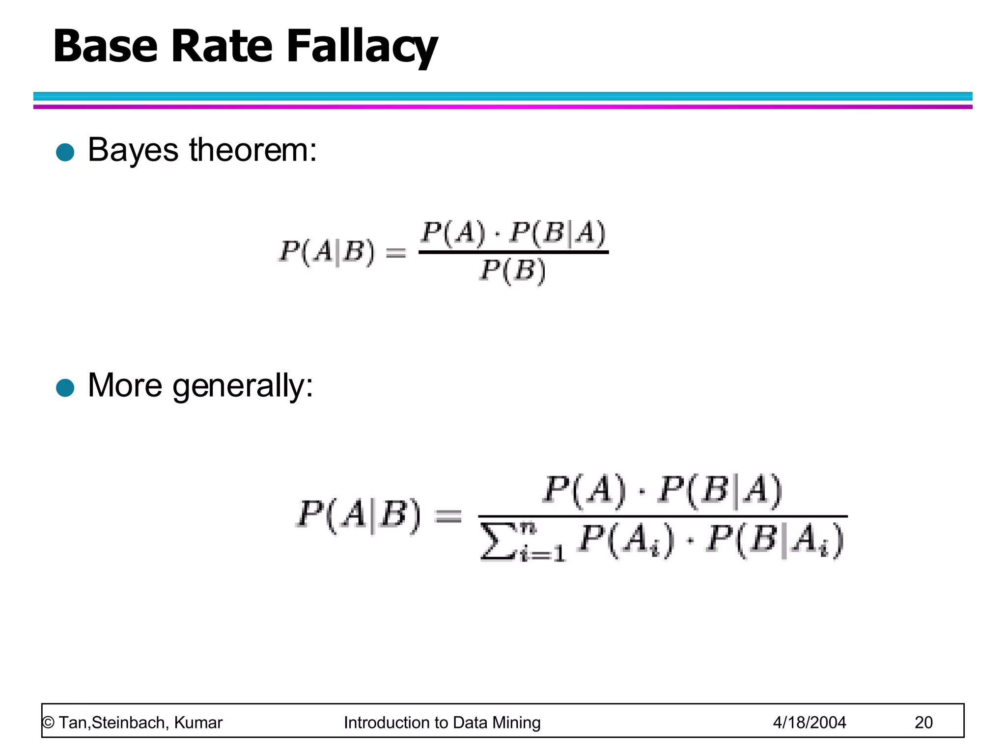
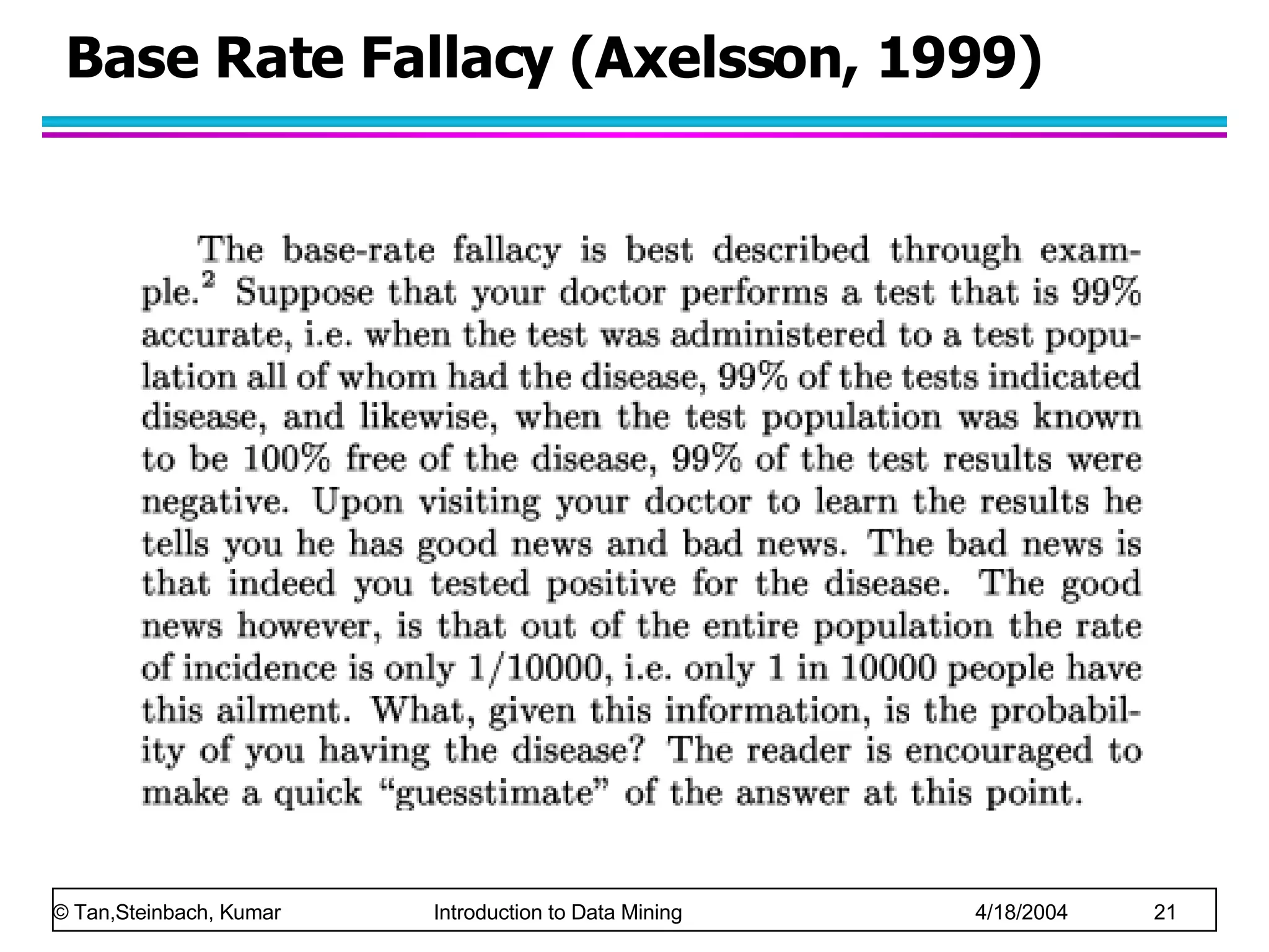
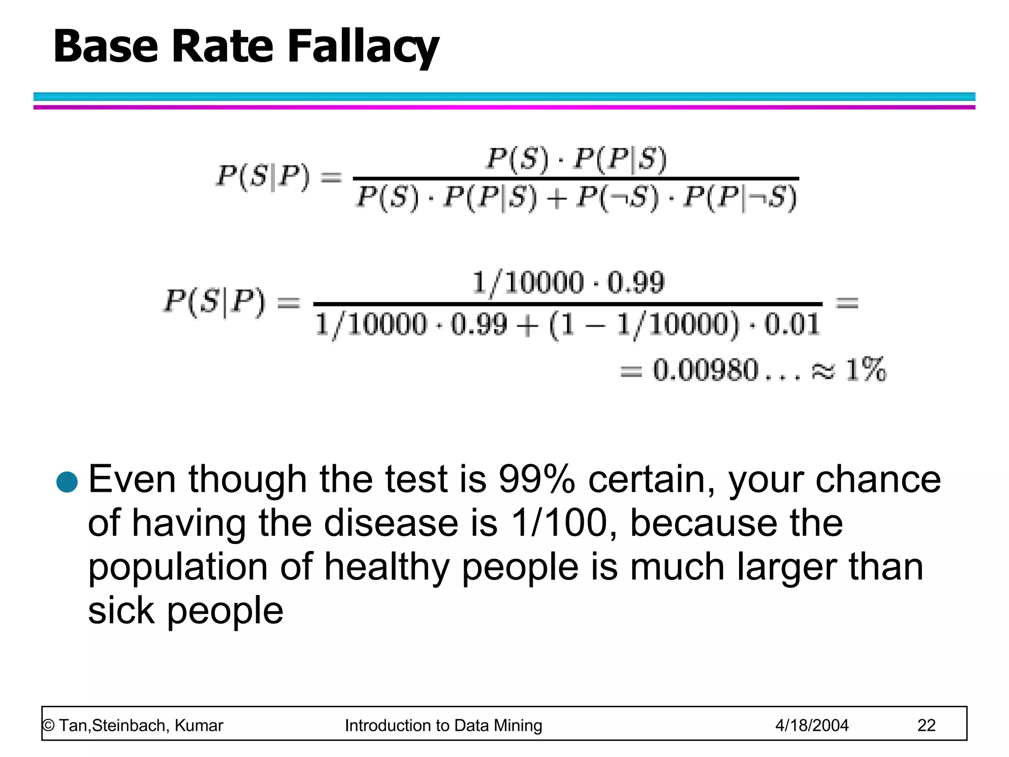
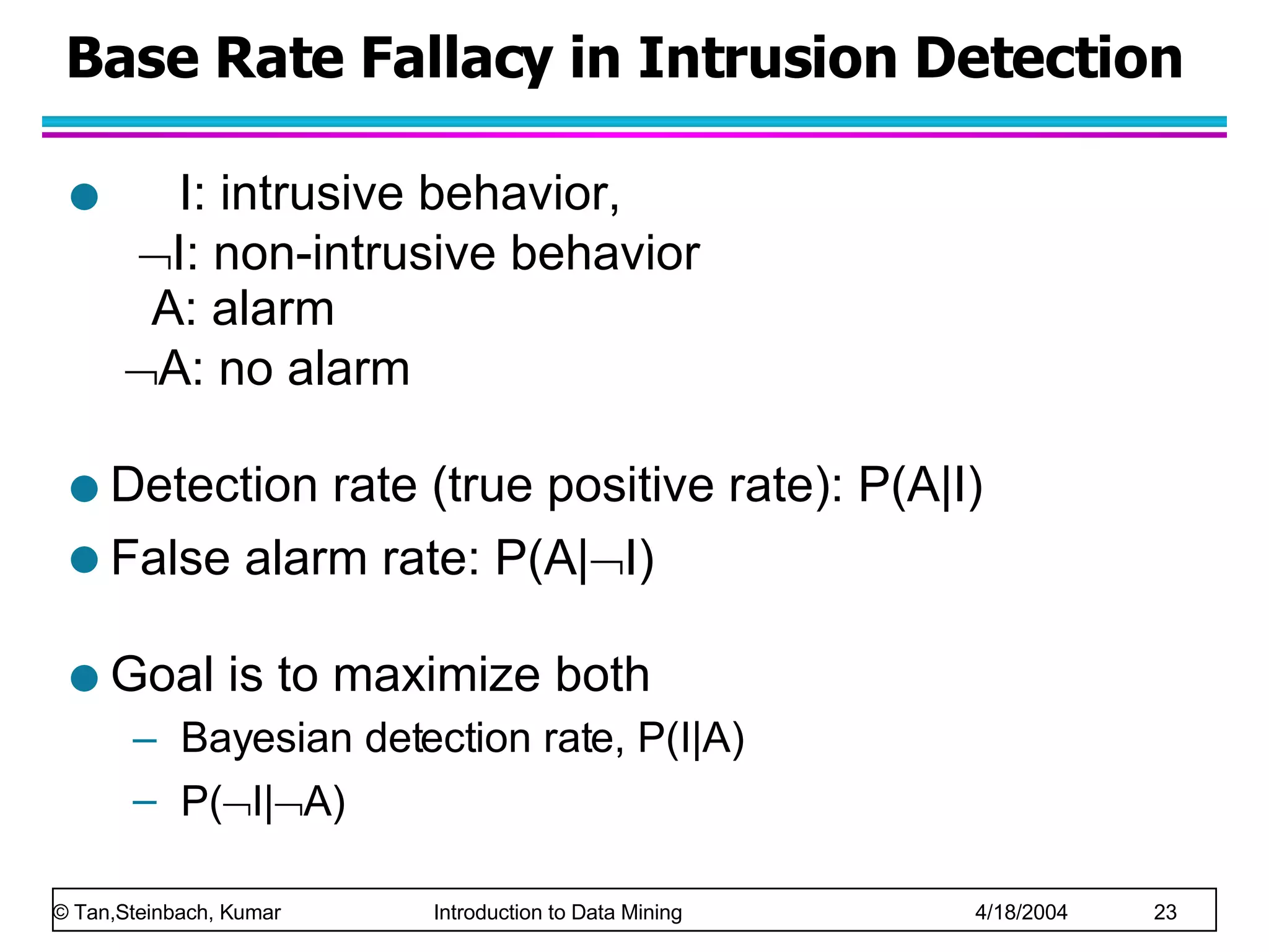
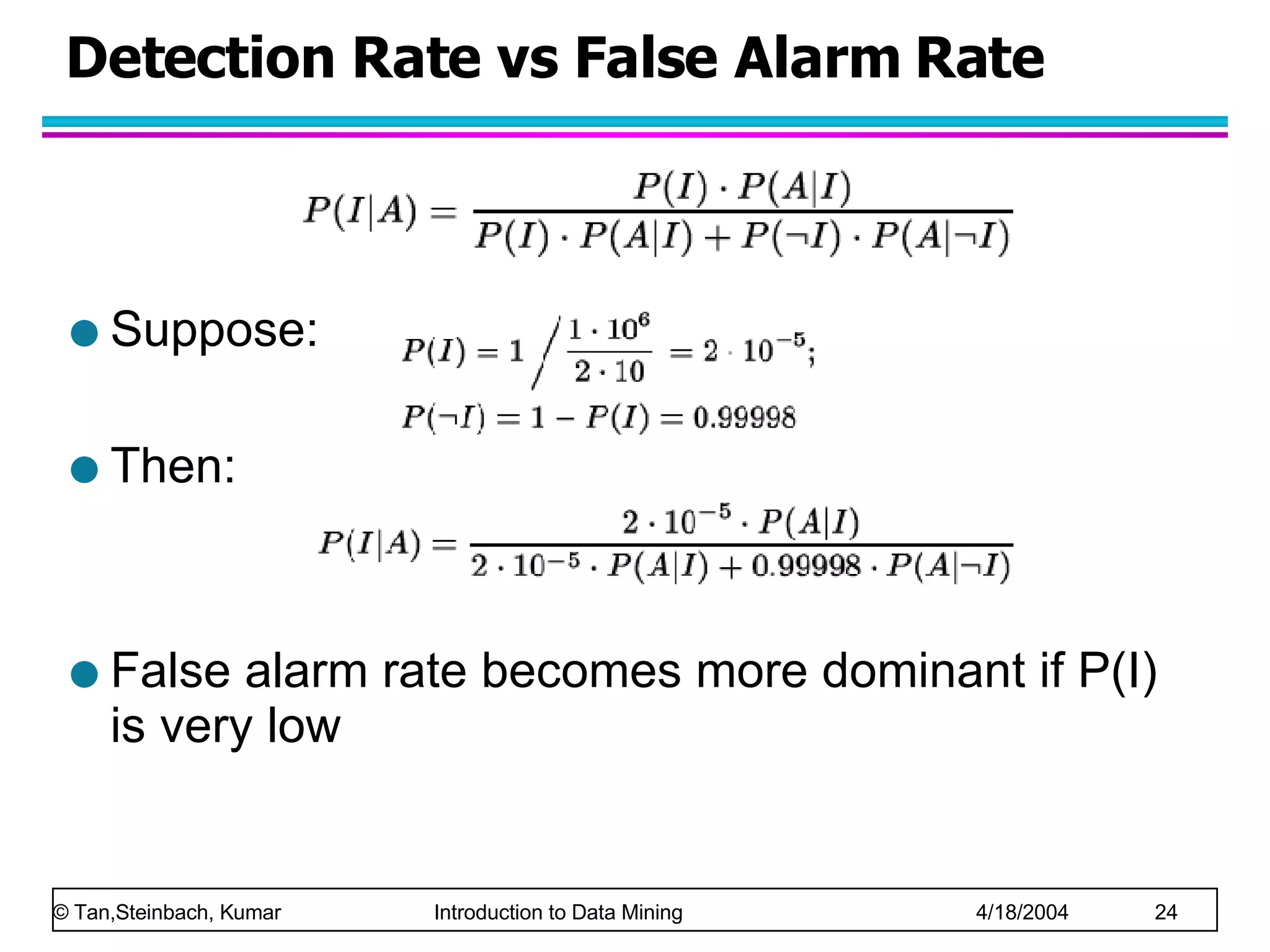
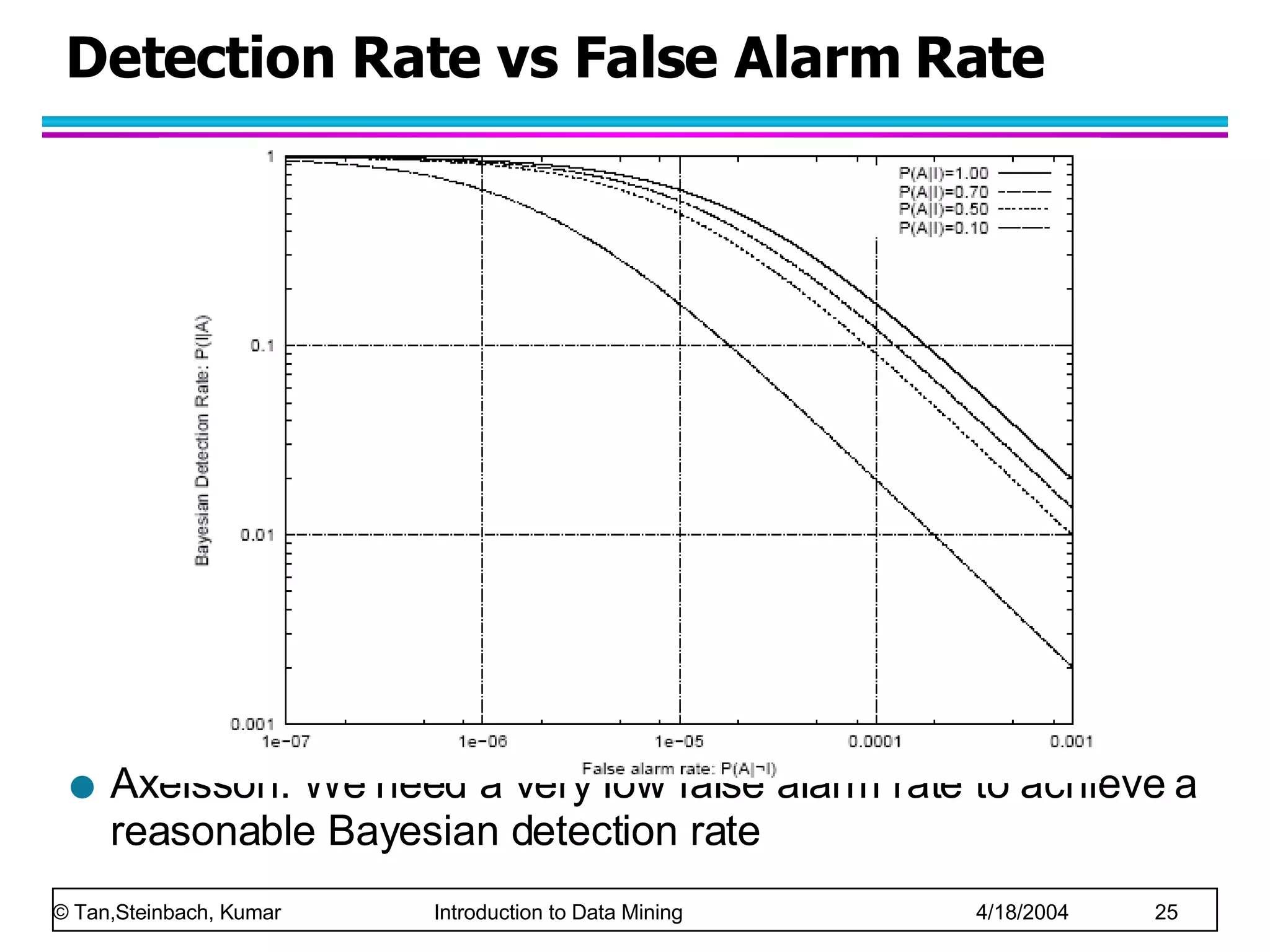
Data Mining Anomaly Detection Lecture Notes for Chapter 10 Introduction to Data Mining by Tan, Steinbach, Kumar © Tan,Steinbach, Kumar Introduction to Data Mining 4/18/2004

Anomaly/Outlier Detection What are anomalies/outliers? The set of data points that are considerably different than the remainder of the data Variants of Anomaly/Outlier Detection Problems Given a database D, find all the data points x  D with anomaly scores greater than some threshold t Given a database D, find all the data points x  D having the top-n largest anomaly scores f( x ) Given a database D, containing mostly normal (but unlabeled) data points, and a test point x , compute the anomaly score of x with respect to D Applications: Credit card fraud detection, telecommunication fraud detection, network intrusion detection, fault detection

Importance of Anomaly Detection Ozone Depletion History In 1985 three researchers (Farman, Gardinar and Shanklin) were puzzled by data gathered by the British Antarctic Survey showing that ozone levels for Antarctica had dropped 10% below normal levels Why did the Nimbus 7 satellite, which had instruments aboard for recording ozone levels, not record similarly low ozone concentrations? The ozone concentrations recorded by the satellite were so low they were being treated as outliers by a computer program and discarded! Sources: http://exploringdata.cqu.edu.au/ozone.html http://www.epa.gov/ozone/science/hole/size.html

Anomaly Detection Challenges How many outliers are there in the data? Method is unsupervised Validation can be quite challenging (just like for clustering) Finding needle in a haystack Working assumption: There are considerably more “normal” observations than “abnormal” observations (outliers/anomalies) in the data

Anomaly Detection Schemes General Steps Build a profile of the “normal” behavior Profile can be patterns or summary statistics for the overall population Use the “normal” profile to detect anomalies Anomalies are observations whose characteristics differ significantly from the normal profile Types of anomaly detection schemes Graphical & Statistical-based Distance-based Model-based

Graphical Approaches Boxplot (1-D), Scatter plot (2-D), Spin plot (3-D) Limitations Time consuming Subjective

Convex Hull Method Extreme points are assumed to be outliers Use convex hull method to detect extreme values What if the outlier occurs in the middle of the data?

Statistical Approaches Assume a parametric model describing the distribution of the data (e.g., normal distribution) Apply a statistical test that depends on Data distribution Parameter of distribution (e.g., mean, variance) Number of expected outliers (confidence limit)

Grubbs’ Test Detect outliers in univariate data Assume data comes from normal distribution Detects one outlier at a time, remove the outlier, and repeat H 0 : There is no outlier in data H A : There is at least one outlier Grubbs’ test statistic: Reject H 0 if:

Statistical-based – Likelihood Approach Assume the data set D contains samples from a mixture of two probability distributions: M (majority distribution) A (anomalous distribution) General Approach: Initially, assume all the data points belong to M Let L t (D) be the log likelihood of D at time t For each point x t that belongs to M, move it to A Let L t+1 (D) be the new log likelihood. Compute the difference,  = L t (D) – L t+1 (D) If  > c (some threshold), then x t is declared as an anomaly and moved permanently from M to A

Statistical-based – Likelihood Approach Data distribution, D = (1 –  ) M +  A M is a probability distribution estimated from data Can be based on any modeling method (naïve Bayes, maximum entropy, etc) A is initially assumed to be uniform distribution Likelihood at time t:

Limitations of Statistical Approaches Most of the tests are for a single attribute In many cases, data distribution may not be known For high dimensional data, it may be difficult to estimate the true distribution

Distance-based Approaches Data is represented as a vector of features Three major approaches Nearest-neighbor based Density based Clustering based

Nearest-Neighbor Based Approach Approach: Compute the distance between every pair of data points There are various ways to define outliers: Data points for which there are fewer than p neighboring points within a distance D The top n data points whose distance to the kth nearest neighbor is greatest The top n data points whose average distance to the k nearest neighbors is greatest

Outliers in Lower Dimensional Projection In high-dimensional space, data is sparse and notion of proximity becomes meaningless Every point is an almost equally good outlier from the perspective of proximity-based definitions Lower-dimensional projection methods A point is an outlier if in some lower dimensional projection, it is present in a local region of abnormally low density

Outliers in Lower Dimensional Projection Divide each attribute into  equal-depth intervals Each interval contains a fraction f = 1/  of the records Consider a k-dimensional cube created by picking grid ranges from k different dimensions If attributes are independent, we expect region to contain a fraction f k of the records If there are N points, we can measure sparsity of a cube D as: Negative sparsity indicates cube contains smaller number of points than expected

Example N=100,  = 5, f = 1/5 = 0.2, N  f 2 = 4

Density-based: LOF approach For each point, compute the density of its local neighborhood Compute local outlier factor (LOF) of a sample p as the average of the ratios of the density of sample p and the density of its nearest neighbors Outliers are points with largest LOF value In the NN approach, p 2 is not considered as outlier, while LOF approach find both p 1 and p 2 as outliers p 2  p 1 

Clustering-Based Basic idea: Cluster the data into groups of different density Choose points in small cluster as candidate outliers Compute the distance between candidate points and non-candidate clusters. If candidate points are far from all other non-candidate points, they are outliers

Base Rate Fallacy Bayes theorem: More generally:

Base Rate Fallacy (Axelsson, 1999)

Base Rate Fallacy Even though the test is 99% certain, your chance of having the disease is 1/100, because the population of healthy people is much larger than sick people

Base Rate Fallacy in Intrusion Detection I: intrusive behavior,  I: non-intrusive behavior A: alarm  A: no alarm Detection rate (true positive rate): P(A|I) False alarm rate: P(A|  I) Goal is to maximize both Bayesian detection rate, P(I|A) P(  I|  A)

Detection Rate vs False Alarm Rate Suppose: Then: False alarm rate becomes more dominant if P(I) is very low

Detection Rate vs False Alarm Rate Axelsson: We need a very low false alarm rate to achieve a reasonable Bayesian detection rate

Chap10 Anomaly Detection

More Related Content

What's hot

Viewers also liked

Similar to Chap10 Anomaly Detection

Recently uploaded

Chap10 Anomaly Detection