Download as PDF, PPTX

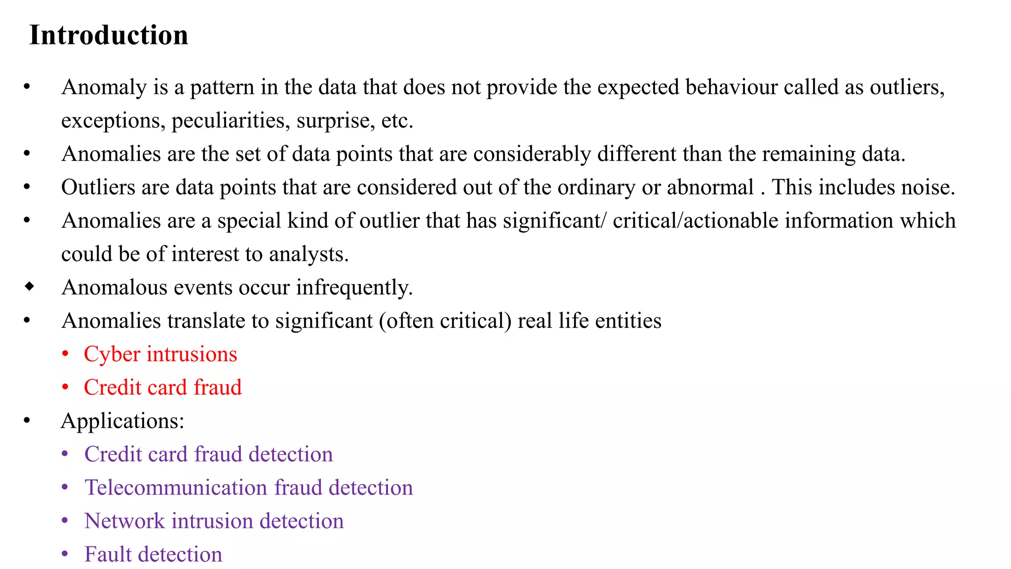
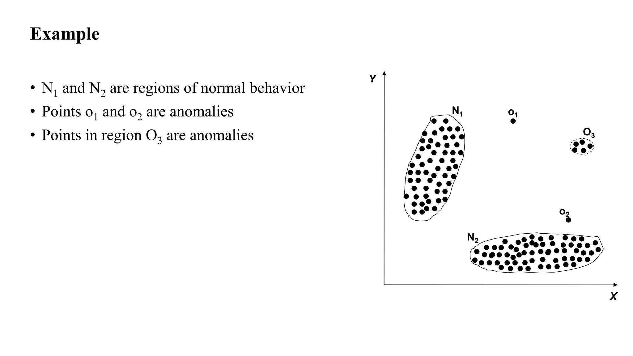
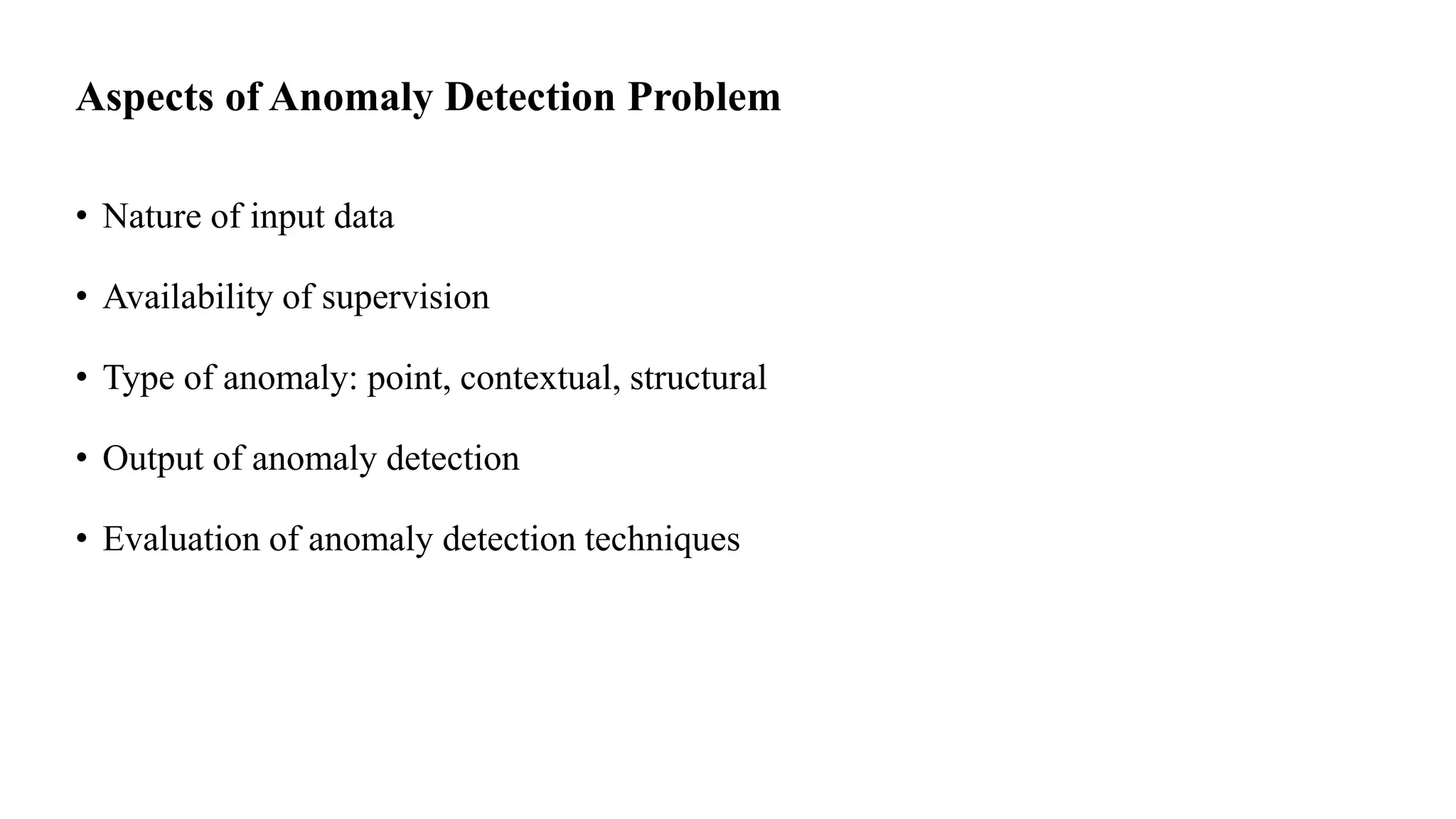
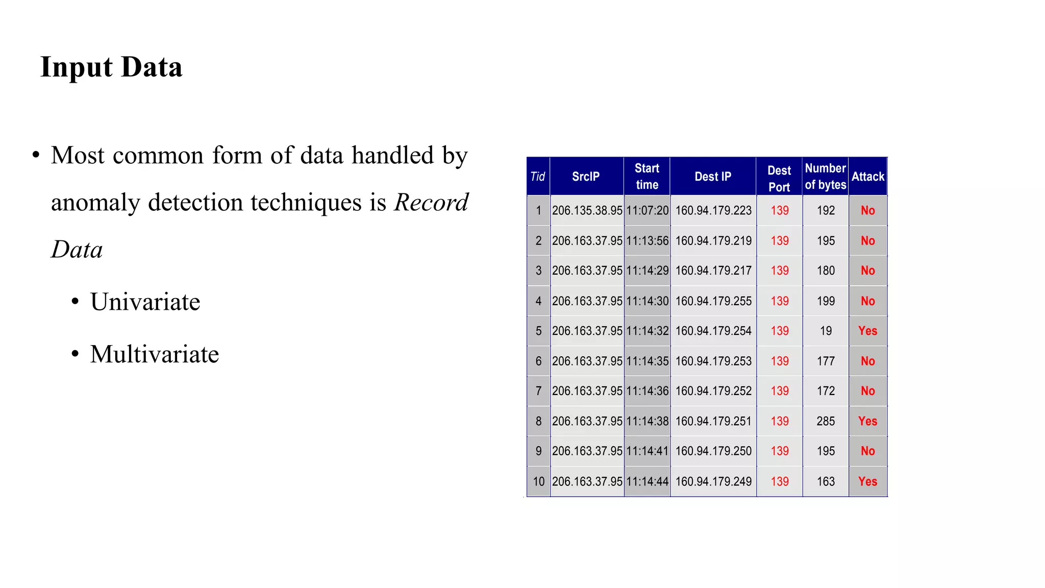

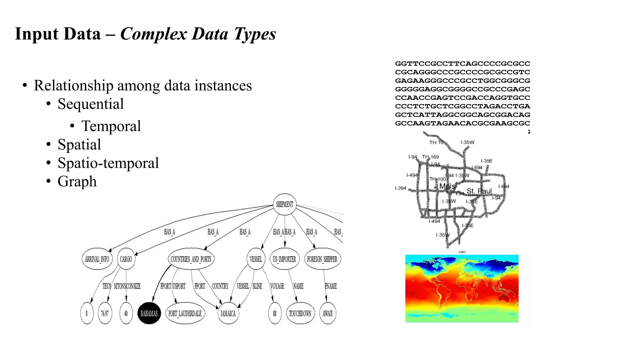
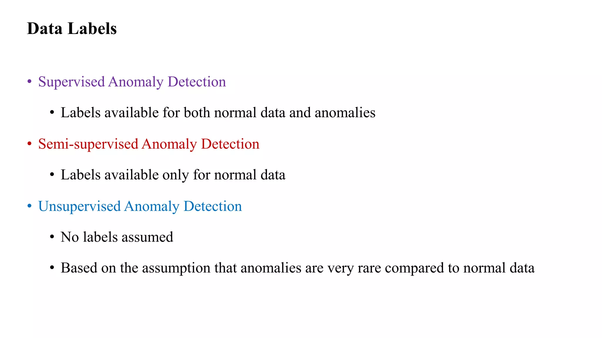

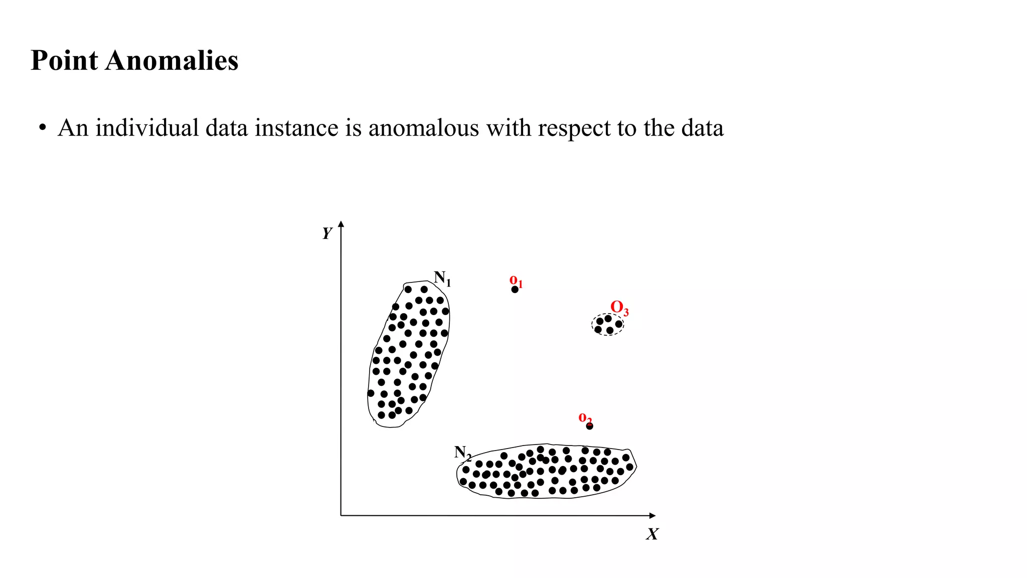
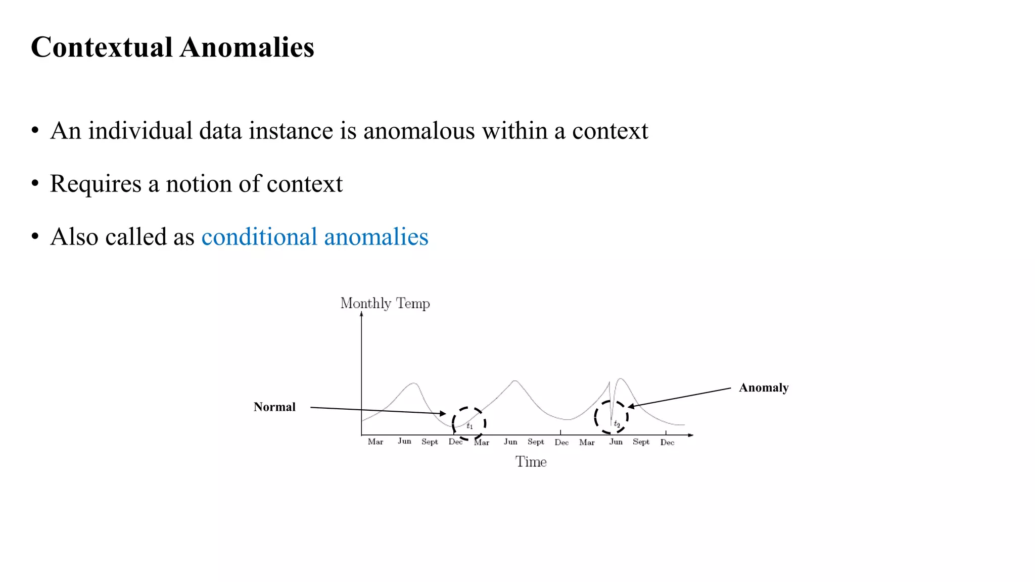
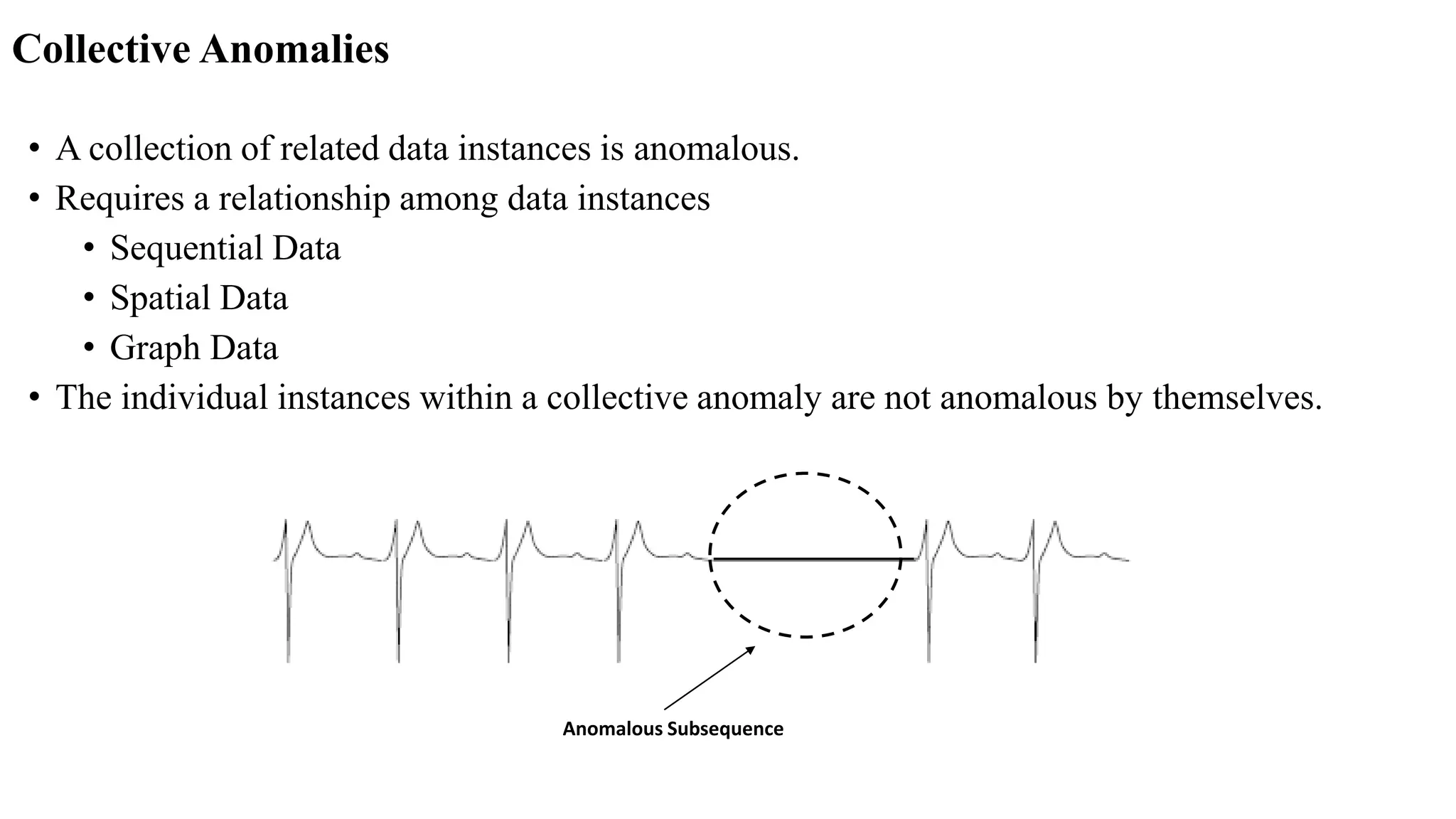
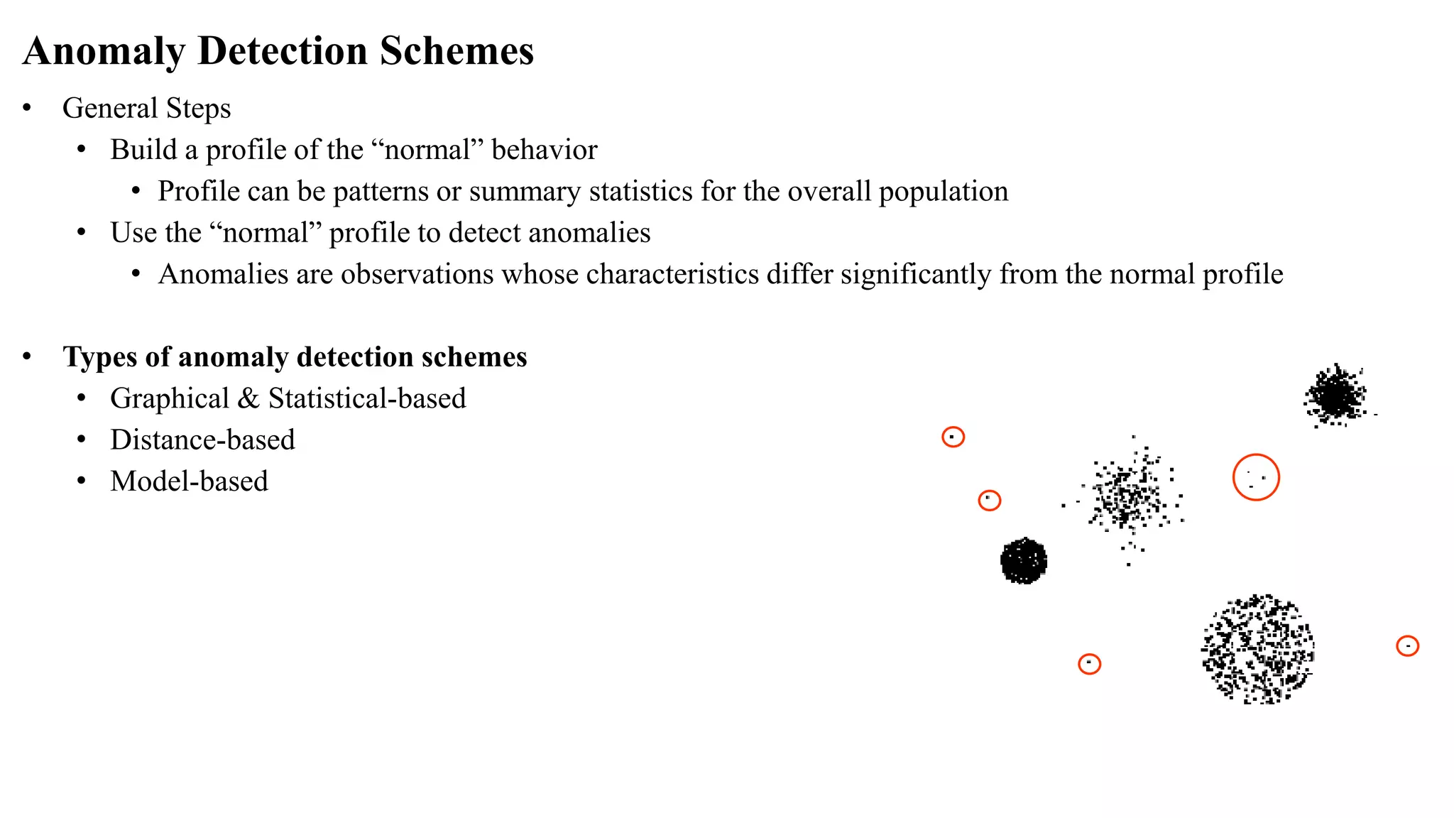

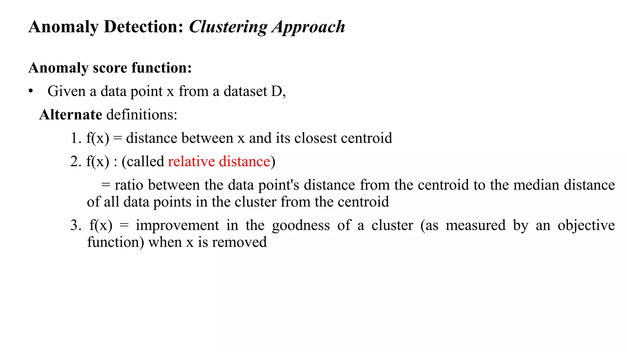


Anomaly detection techniques are used to identify rare items, events or observations which raise suspicions by differing significantly from the majority of the data. There are various types of anomalies including point anomalies, contextual anomalies and collective anomalies. Anomaly detection algorithms typically build a model of normal behavior and then label new data as normal or anomalous based on how well it fits the model. Common techniques include clustering, statistical methods and distance-based approaches. Applications include fraud detection, system failure diagnosis and cybersecurity.