Downloaded 935 times
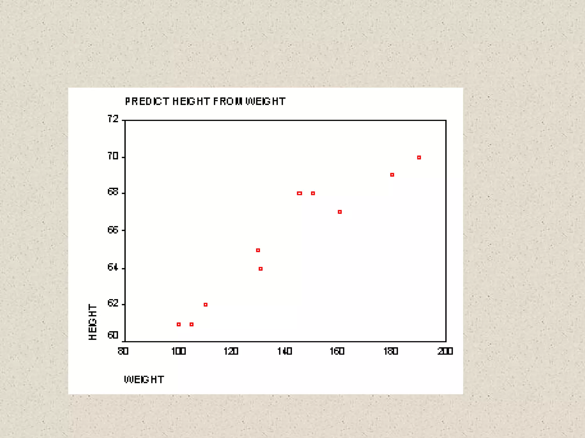
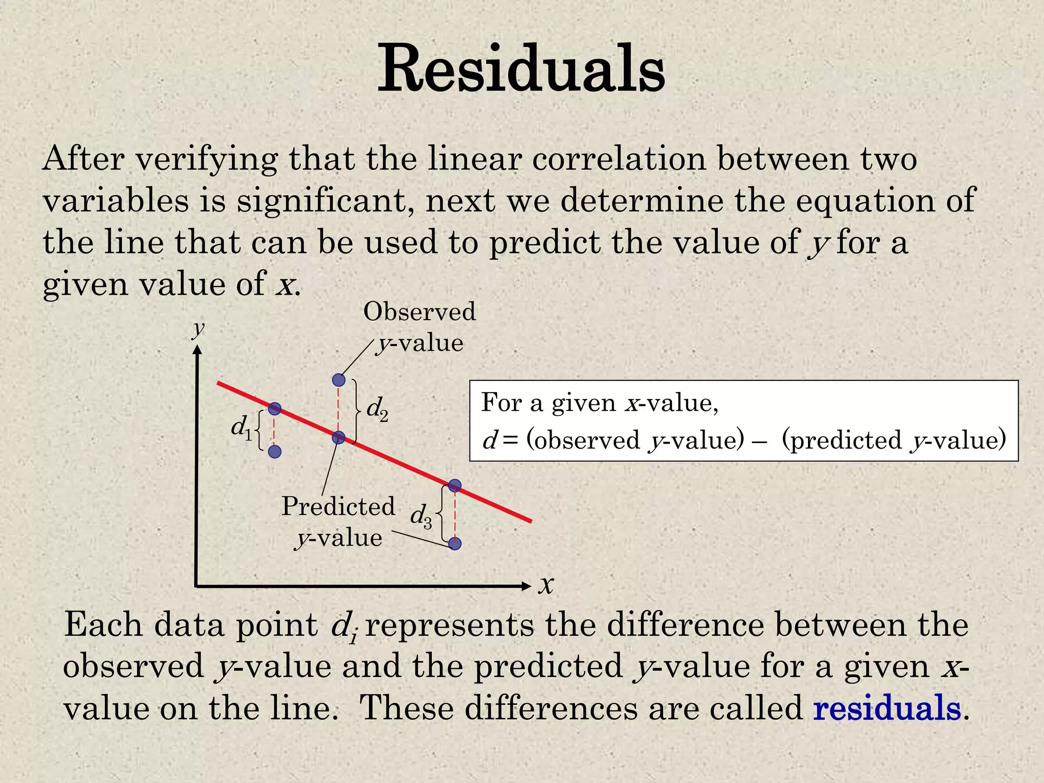
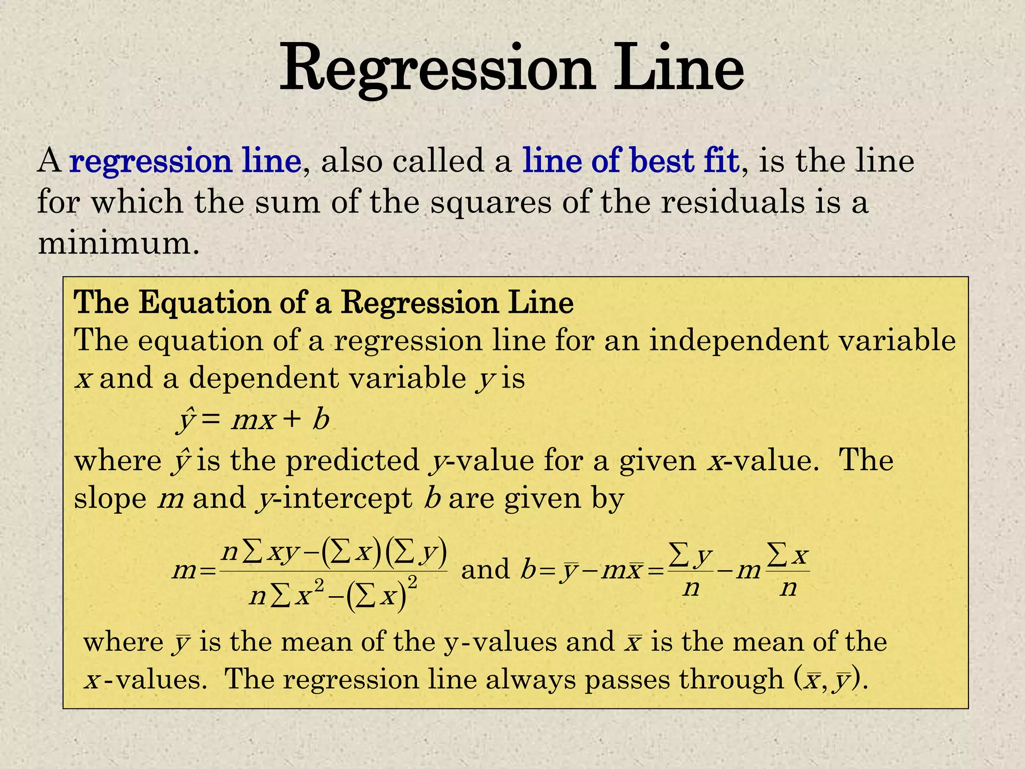
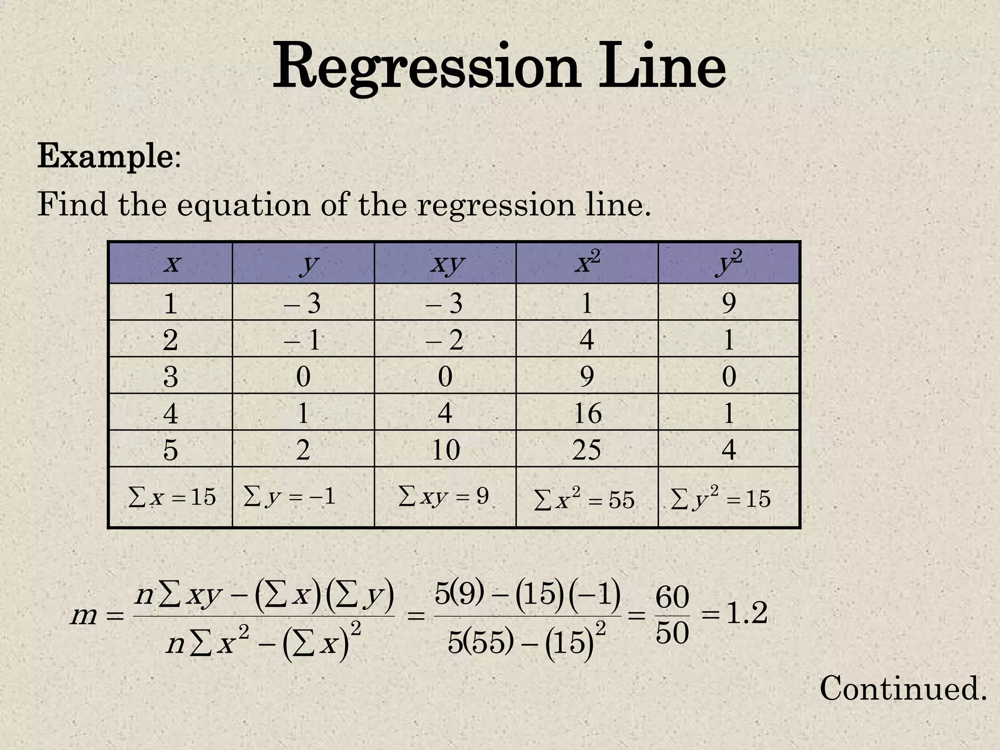
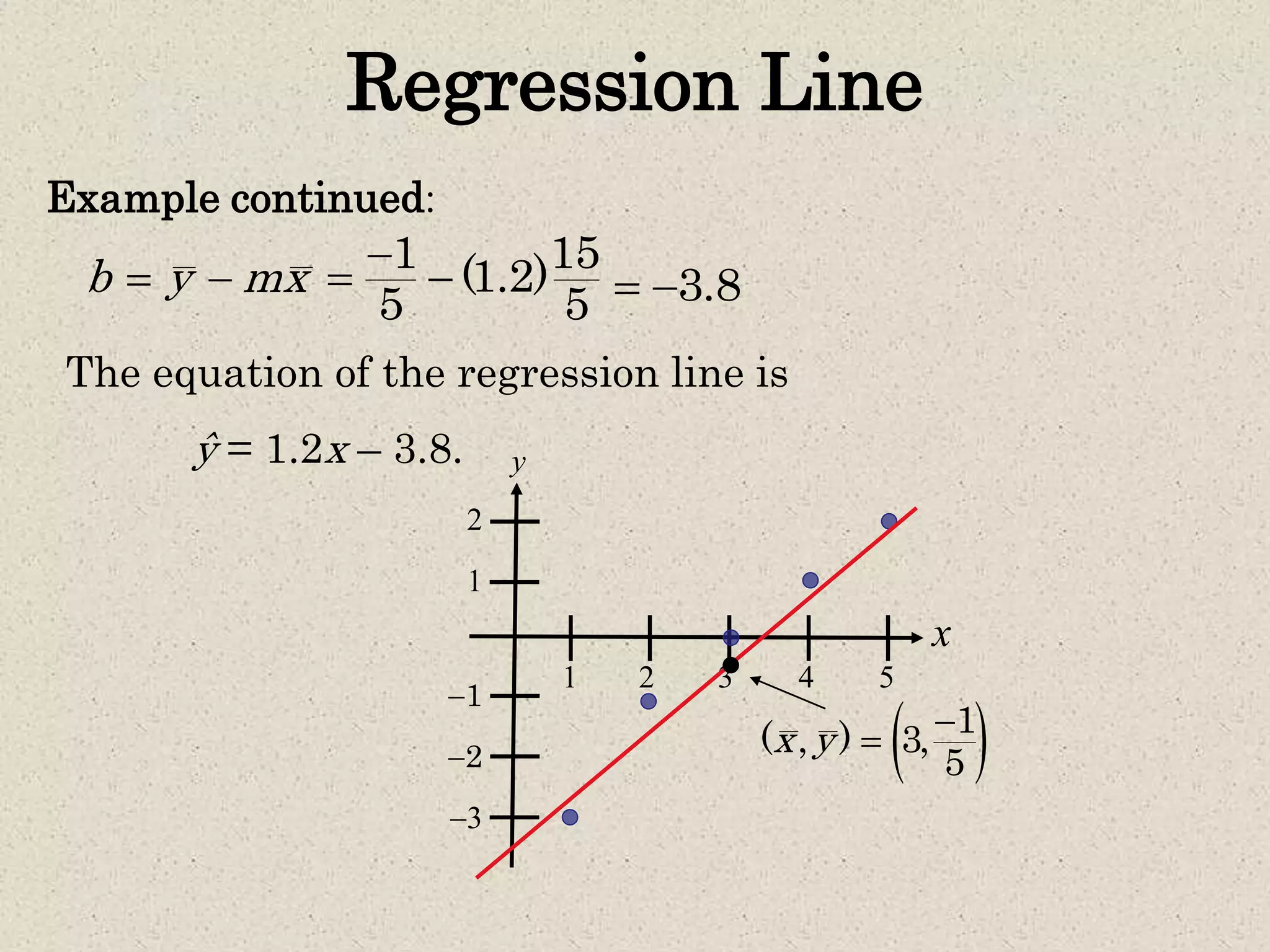
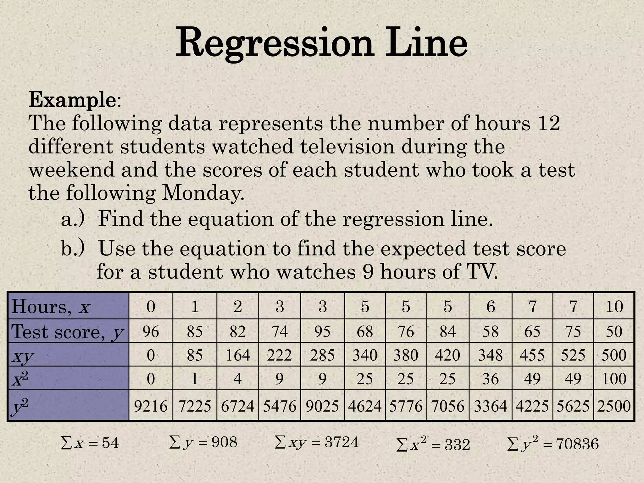
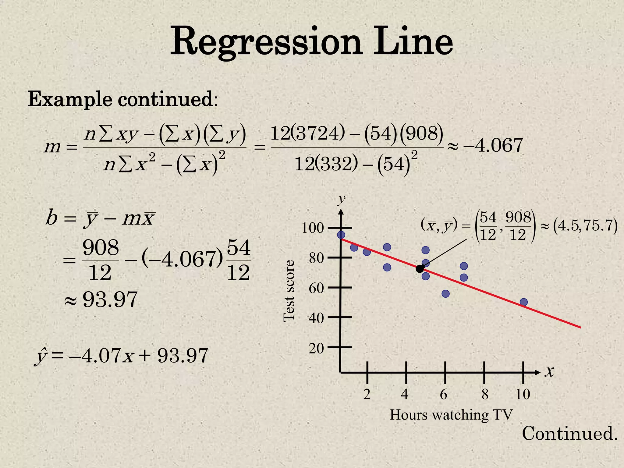
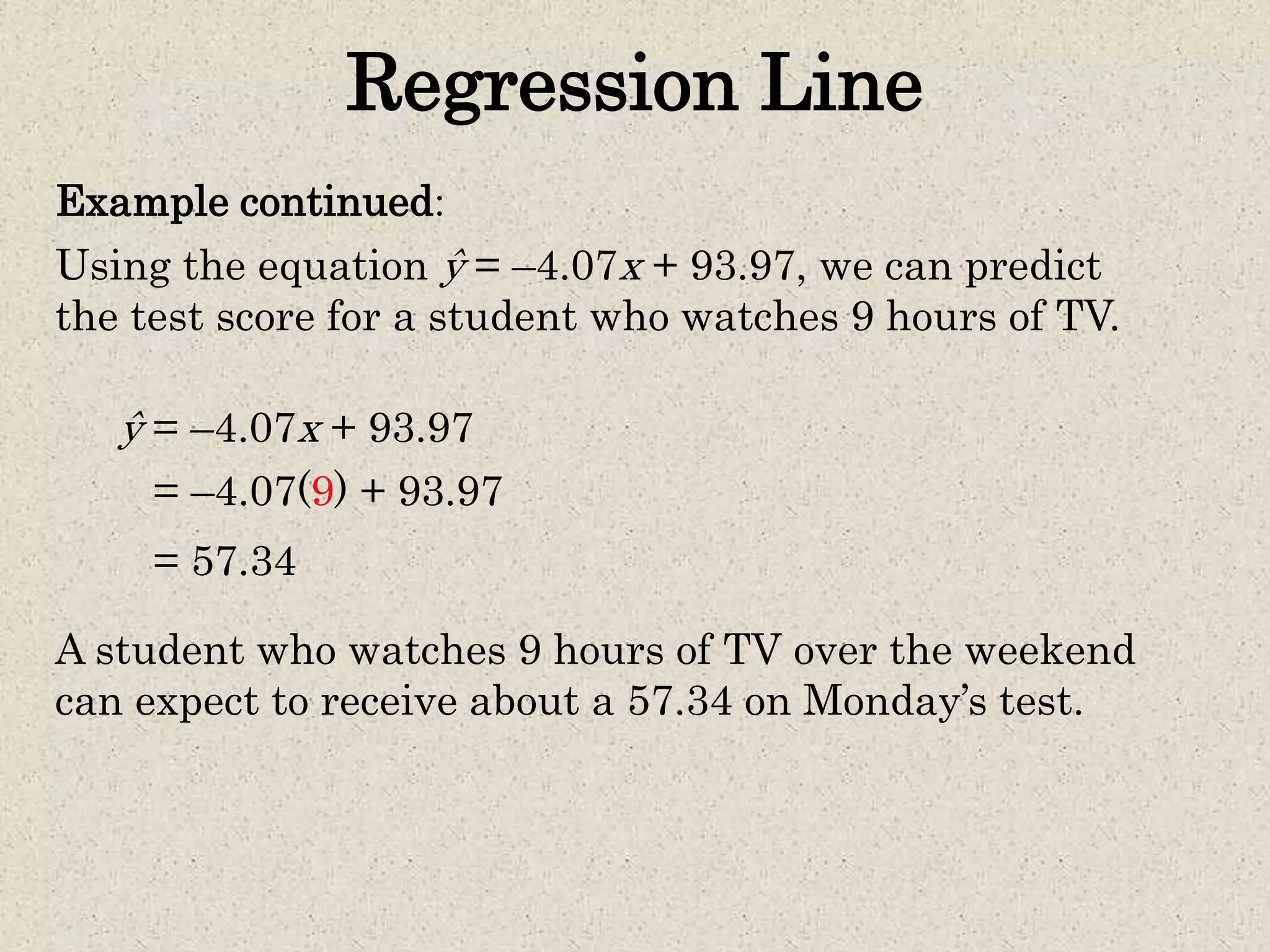
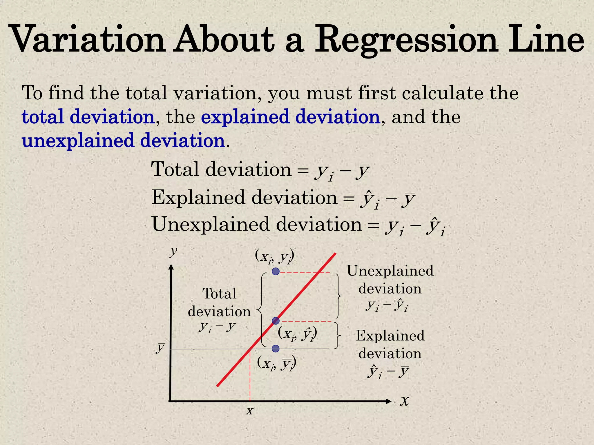
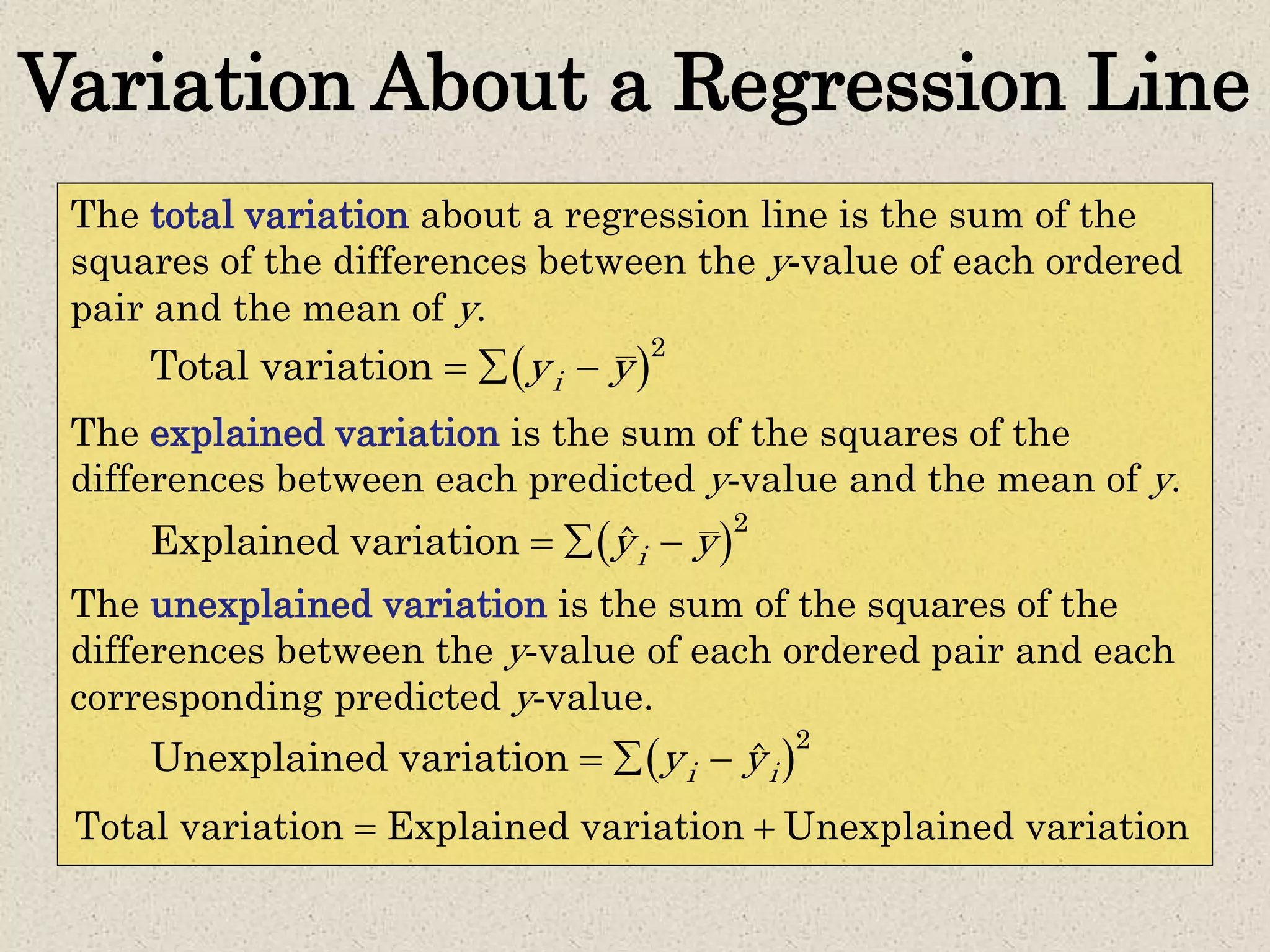
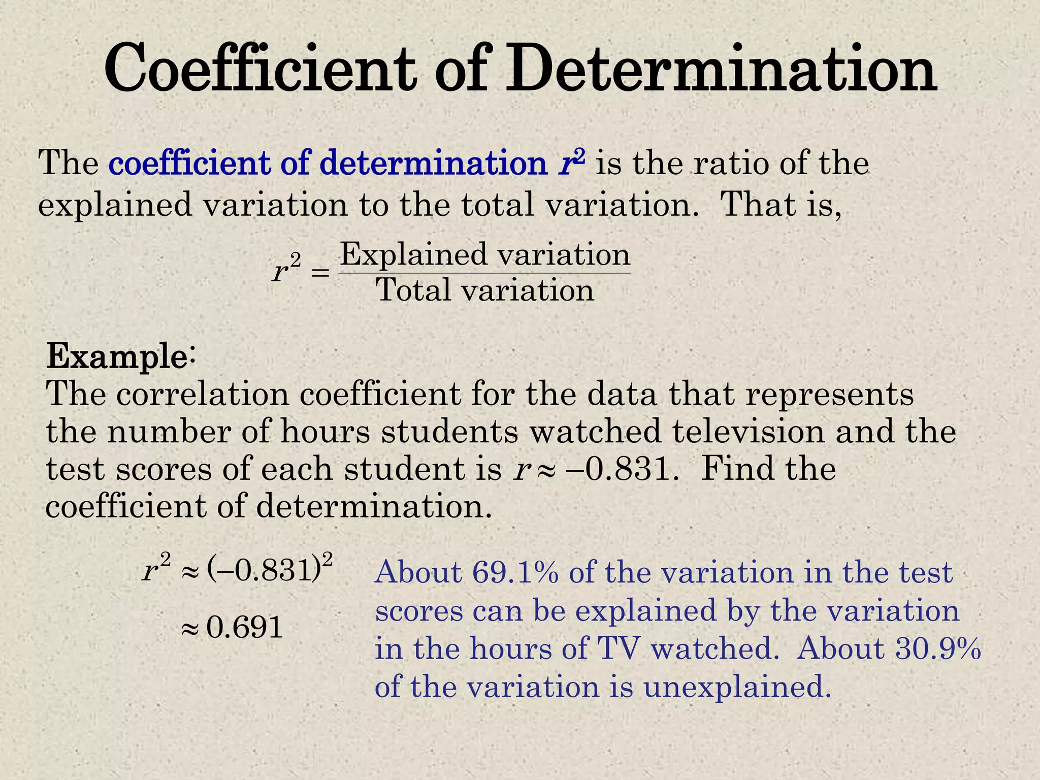
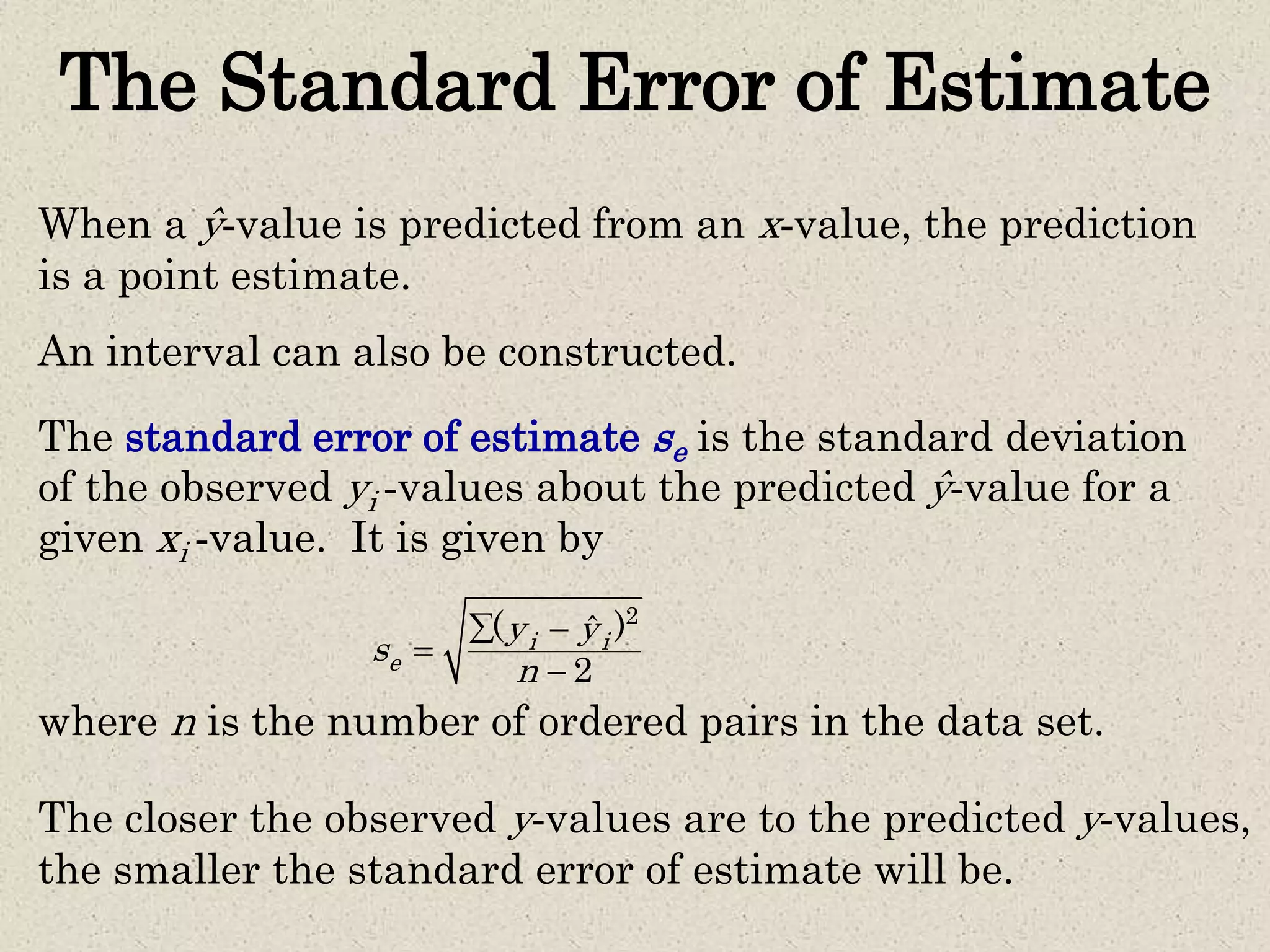
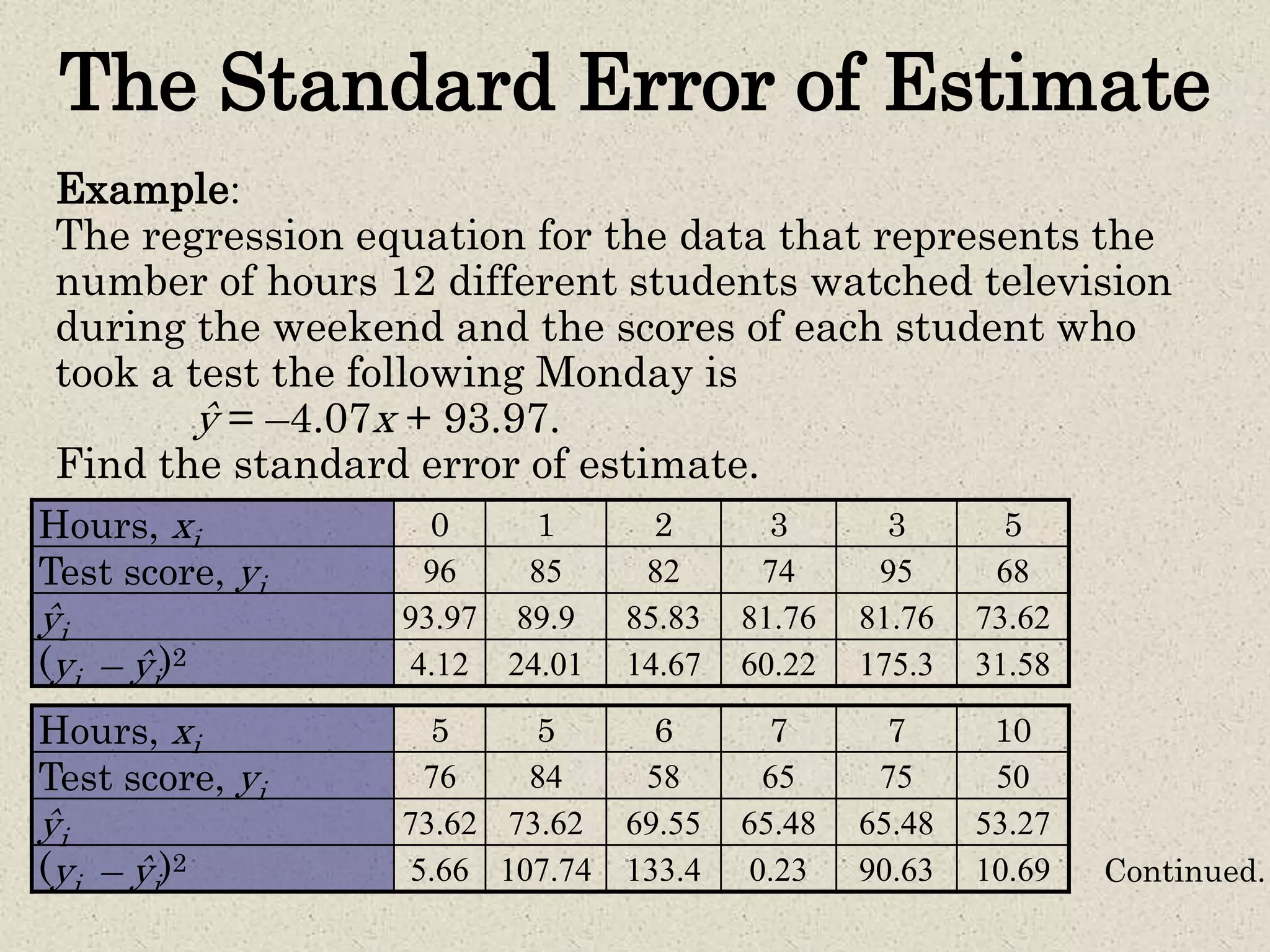
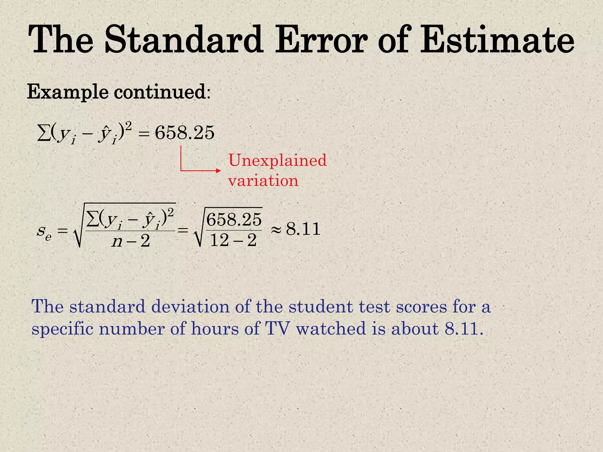
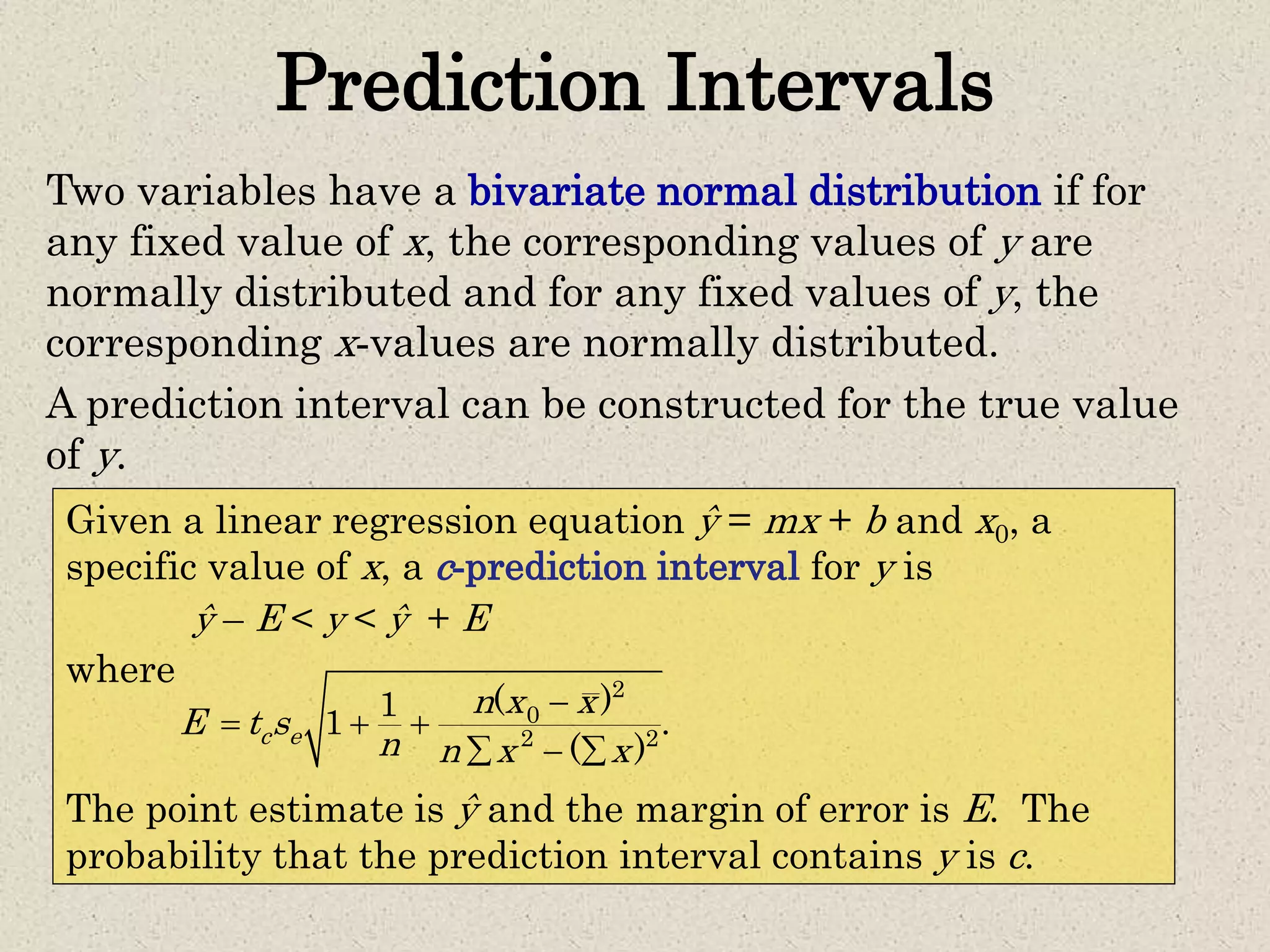
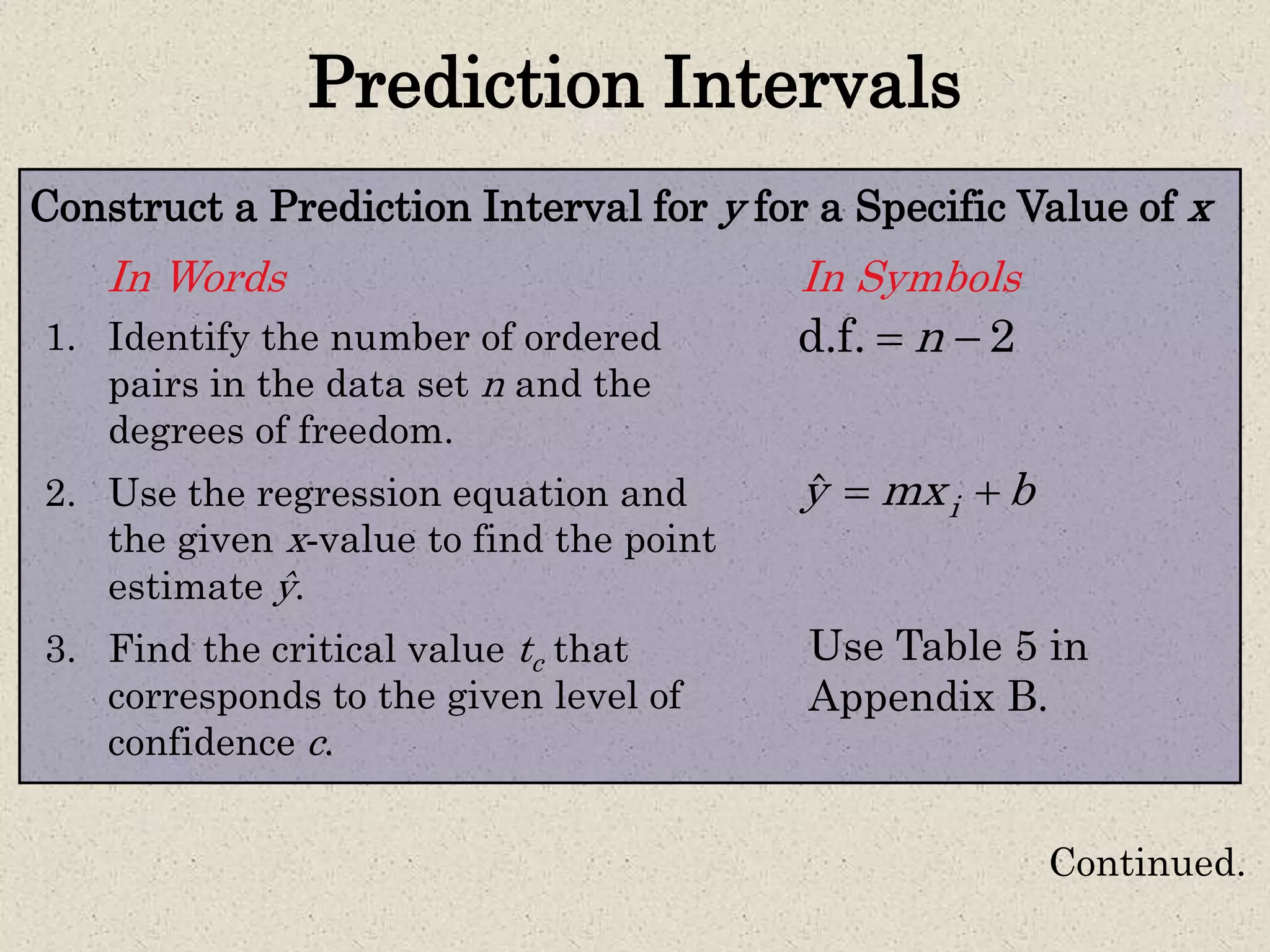
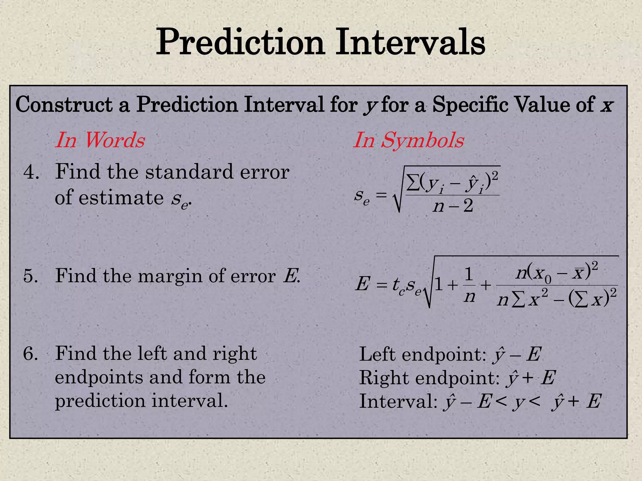
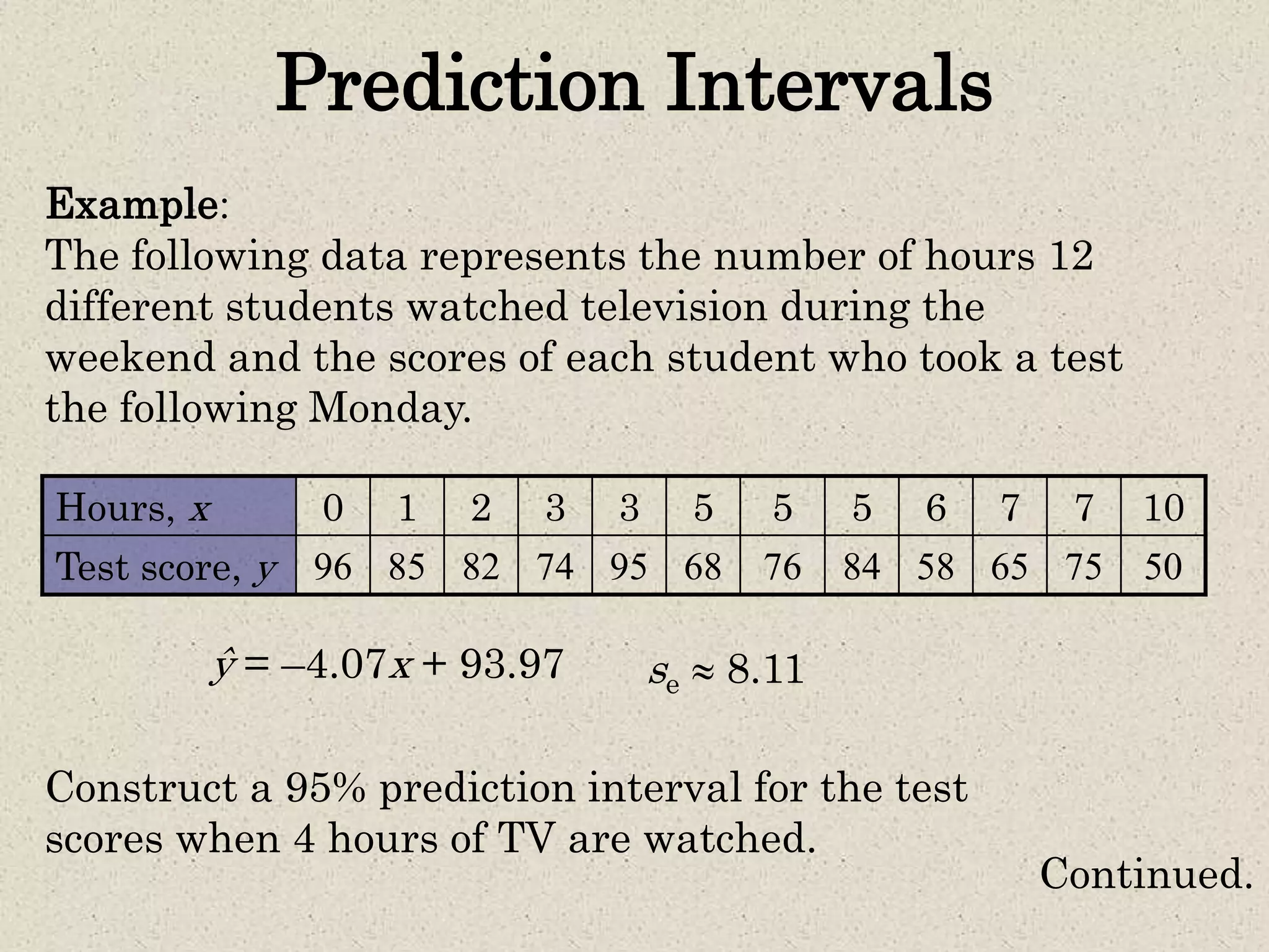
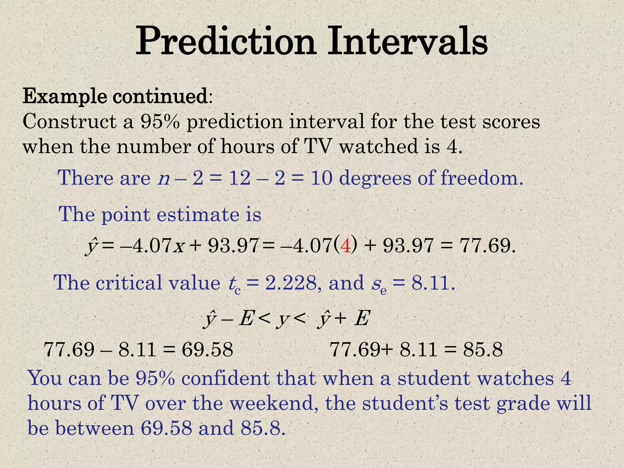
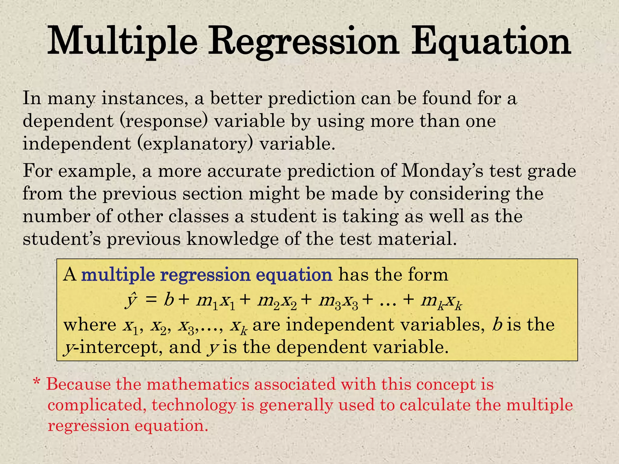


- Simple linear regression is used to predict values of one variable (dependent variable) given known values of another variable (independent variable). - A regression line is fitted through the data points to minimize the deviations between the observed and predicted dependent variable values. The equation of this line allows predicting dependent variable values for given independent variable values. - The coefficient of determination (R2) indicates how much of the total variation in the dependent variable is explained by the regression line. The standard error of estimate provides a measure of how far the observed data points deviate from the regression line on average. - Prediction intervals can be constructed around predicted dependent variable values to indicate the uncertainty in predictions for a given confidence level, based on the