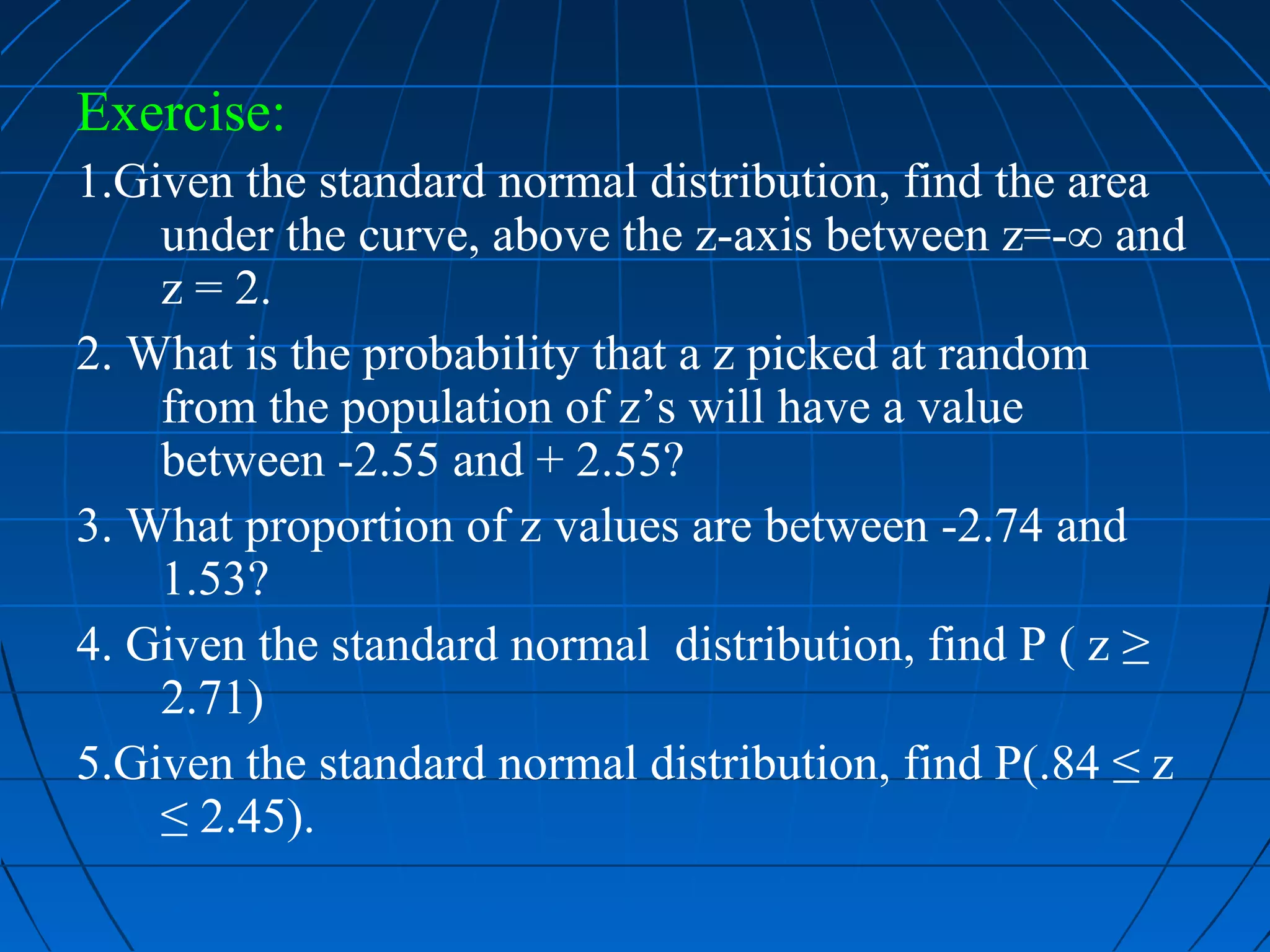
Lecture Series on
  Biostatistics

                No. Bio-Stat_9
               Date – 01.02.2009


  Some Basic Probability Concept
   and Probability Distribution
                       By
           Dr. Bijaya Bhusan Nanda,
       M.Sc. (Gold Medalist), Ph. D. (Stat.)
Continuous Probability Distribution
Continuous variable:
   Assumes any value within a specified
    interval/range.
   Consequently any two values within a specified
    interval, there exists an infinite number of values.
   As the number of observation, n, approaches
    infinite and the width of the class interval
    approaches zero, the frequency polygon approaches
    smooth curve.
   Such smooth curves are used to represent
    graphically the distribution of continuous random
    variable
   This has some important consequences when we deal with
    probability distributions.
   The total area under the curve is equal to 1 as in the case
    of the histogram.
   The relative frequency of occurrence of values between
    any two points on the x-axis is equal to the total area
    bounded by the curve, the x-axis and the perpendicular
    lines erected at the two points.

        f (x)


                                    a     b            x
Graph of a continuous distribution showing area between a and b
Definition of probability distribution:
   A density function is a formula used to represent the
    probability distribution of a continuous random
    variable.
   This is a nonnegative function f (x) of the continuous
    r.v, x if the total area bounded by its curve and the x-
    axis is equal to 1 and if the sub area under the curve
    bounded by the curve, the x-axis and perpendiculars
    erected at any two points a and b gives the probability
    that x is between the point a and b.
Normal Distribution( C.F.Gauss, 1777-1855)
 The distribution is frequently called the Gaussian
 distribution.
 It is a relative frequency distribution of errors, such
 errors of measurement. This curve provides an
 adequate model for the relative frequency
 distributions of data collected from many different
 scientific areas.
 The density function for a normal random variable

                                1    − ( x − µ ) 2 / 2σ 2
                     f ( x) =      e
                              σ 2π
   The parameters µ and σ2 are the mean and the
    variance , respectively, of the normal random variable
Characteristics Of The Normal Distribution

    It is symmetrical about its mean, µ.
    The mean, the median, and the mode are all equal.
    The total area under the curve above the x-axis is one
    square unit.
    This characteristic follows that the normal
    distribution is a probability distribution.
   Because of the symmetry already mentioned, 50% of
    the area is to the right of a perpendicular erected at
    the mean, and 50% is to the left.
 If µ = 0 and σ =1 then . The distribution with this
  density function is called the standardized normal
   distribution. The graph of the standardized normal
density distribution is shown in Figure

         0.5
         0.4
         0.3
         0.2
         0.1
          0


                                                                         2
                                           -1


                                                       0.2
                                                             0.8
                                                                   1.4


                                                                             2.6
                                                                                   3.2
               -3.4
                      -2.8
                             -2.2
                                    -1.6


                                                -0.4
   If ‘x’ is a normal random variable with the mean µ
    and variance σ then
    1) the variable        x−µ
                     z=
                           σ
  is the standardized normal random variable.
The equation of pdf for standard normal distribution
                       1
              f (z) =     e –z2 / 2, -∞ < z < ∞
                      √2∏
   Area properties of normal distribution
            P( x − µ ≤ 2σ ) = 0.9544
            P( x − µ ≤ 2σ ) = 0.9544
            P( x − µ ≤ 3σ ) = 0.9973
   Namely, if a population of measurements has
    approximately a normal distribution the probability
    that a random selected observation falls within the
    intervals (µ - σ, µ + σ), (µ - 2σ, µ +2σ), and (µ -
    3σ, µ + 3σ), is approximately 0.6826, 0.9544 and
    0.9973, respectively.
 Normal Distribution Application
Example:1 As a part of a study of Alzeheimer’s disease, reported data that
    are compatible with the hypothesis that brain weights of victims of the
    disease are normally distributed. From the reported data, we may
    compute a mean of 1076.80 grams and a standard deviation of 105.76
    grams. If we assume that these results are applicable to all victims of
    Alzeheimer’s disease, find the probability that a randomly selected victim
    of the disease will have a brain that weighs less than 800 grams.


                                              σ = 105.76


                               800    µ = 1076.80
Solution:
    R.V x ‘Brain weights’ follows a Normal distribution
      with µ=1076.80 and σ = 105.76)
                                                                   x−µ
    The Corresponding Standard Normal Variate                   z=
                                                                    σ
    =      x − 1076.80
       z=
             105.76
We have to find out P (x < 800) i.e P (z
< -2.62). This is the area bounded by
the curve, x axis and to the left of the                  σ=1
perpendicular drawn at z = -2.62.
Thus from the standard normal table
this prob., p= .0044. The probability is .
0044 that a randomly selected patient
will have a brain weight of less than
800 grams.
                                             - 2.62   0
Example: 2
  Suppose it is known that the heights of a certain
  population of individuals are approximately normally
  distributed with a mean of 70 inches and a standard
  deviation of 3 inches. What is the probability that a
  person picked at random from this group will be
  between 65 and 74 inches tall.
Solution: In fig are shown that the distribution of
  heights and the z distribution to which we transform
  the original values to determine the desired
  probabilities. We find the value corresponding to an x
  of 65 by
65-70
z=           = -1.76
       3

                            σ=3


             65
             65        70   74
                            74

                            σ=1


              -1.67     0    1.33
Similarly, for x= 74 we have
                     74-70
                z=            = 1.33
                       3

   The area between -∞ and -1.76 to be .0475 and the area
     between -∞ and 1.33 to be .9082. The area desired is
     the difference between these, .9082- .0475=.8607
   To summarize,
                                       65-70         74-70
         P ( 65 ≤ x ≤ 74) = P     (   3
                                               ≤z≤     3
                                                             )
                           = P (- 1.76 ≤ z ≤ 1.33)
                           = P ( -∞ ≤ z ≤ 1.33) – P (-∞ ≤ z ≤ -1.67)
                             = .9082 - .0475
                             = .8607
The probability asked for in our original question, then, is .8607
Example: 3
  In a population of 10,000 of the people described in
  previous example how many would you expect to be
  6 feet 5 inches tall or taller?
Solution:
  we first find the probability that one person selected
  at random from the population would be 6 feet 5
  inches tall or taller. That is,
                         77-70
                    (
    P ( x ≥ 77 ) = P z ≥ 3       )
                 = P ( z ≥ 2.33 ) = 1 - .9901= .0099
Out of 10,000 people we would expect 10,000 (.0099) =
99 to be 6 feet 5 inches (77 inches tall or taller).
Exercise:
1.Given the standard normal distribution, find the area
    under the curve, above the z-axis between z=-∞ and
    z = 2.
2. What is the probability that a z picked at random
    from the population of z’s will have a value
    between -2.55 and + 2.55?
3. What proportion of z values are between -2.74 and
    1.53?
4. Given the standard normal distribution, find P ( z ≥
    2.71)
5.Given the standard normal distribution, find P(.84 ≤ z
    ≤ 2.45).

Probability concept and Probability distribution_Contd

  • 1.
    Lecture Series on Biostatistics No. Bio-Stat_9 Date – 01.02.2009 Some Basic Probability Concept and Probability Distribution By Dr. Bijaya Bhusan Nanda, M.Sc. (Gold Medalist), Ph. D. (Stat.)
  • 2.
    Continuous Probability Distribution Continuousvariable:  Assumes any value within a specified interval/range.  Consequently any two values within a specified interval, there exists an infinite number of values.  As the number of observation, n, approaches infinite and the width of the class interval approaches zero, the frequency polygon approaches smooth curve.  Such smooth curves are used to represent graphically the distribution of continuous random variable
  • 3.
    This has some important consequences when we deal with probability distributions.  The total area under the curve is equal to 1 as in the case of the histogram.  The relative frequency of occurrence of values between any two points on the x-axis is equal to the total area bounded by the curve, the x-axis and the perpendicular lines erected at the two points. f (x) a b x Graph of a continuous distribution showing area between a and b
  • 4.
    Definition of probabilitydistribution:  A density function is a formula used to represent the probability distribution of a continuous random variable.  This is a nonnegative function f (x) of the continuous r.v, x if the total area bounded by its curve and the x- axis is equal to 1 and if the sub area under the curve bounded by the curve, the x-axis and perpendiculars erected at any two points a and b gives the probability that x is between the point a and b.
  • 5.
    Normal Distribution( C.F.Gauss,1777-1855)  The distribution is frequently called the Gaussian distribution.  It is a relative frequency distribution of errors, such errors of measurement. This curve provides an adequate model for the relative frequency distributions of data collected from many different scientific areas.  The density function for a normal random variable 1 − ( x − µ ) 2 / 2σ 2 f ( x) = e σ 2π  The parameters µ and σ2 are the mean and the variance , respectively, of the normal random variable
  • 6.
    Characteristics Of TheNormal Distribution  It is symmetrical about its mean, µ.  The mean, the median, and the mode are all equal.  The total area under the curve above the x-axis is one square unit.  This characteristic follows that the normal distribution is a probability distribution.  Because of the symmetry already mentioned, 50% of the area is to the right of a perpendicular erected at the mean, and 50% is to the left.
  • 7.
     If µ= 0 and σ =1 then . The distribution with this density function is called the standardized normal distribution. The graph of the standardized normal density distribution is shown in Figure 0.5 0.4 0.3 0.2 0.1 0 2 -1 0.2 0.8 1.4 2.6 3.2 -3.4 -2.8 -2.2 -1.6 -0.4
  • 8.
    If ‘x’ is a normal random variable with the mean µ and variance σ then 1) the variable x−µ z= σ is the standardized normal random variable. The equation of pdf for standard normal distribution 1 f (z) = e –z2 / 2, -∞ < z < ∞ √2∏  Area properties of normal distribution P( x − µ ≤ 2σ ) = 0.9544 P( x − µ ≤ 2σ ) = 0.9544 P( x − µ ≤ 3σ ) = 0.9973
  • 9.
    Namely, if a population of measurements has approximately a normal distribution the probability that a random selected observation falls within the intervals (µ - σ, µ + σ), (µ - 2σ, µ +2σ), and (µ - 3σ, µ + 3σ), is approximately 0.6826, 0.9544 and 0.9973, respectively.
  • 10.
     Normal DistributionApplication Example:1 As a part of a study of Alzeheimer’s disease, reported data that are compatible with the hypothesis that brain weights of victims of the disease are normally distributed. From the reported data, we may compute a mean of 1076.80 grams and a standard deviation of 105.76 grams. If we assume that these results are applicable to all victims of Alzeheimer’s disease, find the probability that a randomly selected victim of the disease will have a brain that weighs less than 800 grams. σ = 105.76 800 µ = 1076.80
  • 11.
    Solution: R.V x ‘Brain weights’ follows a Normal distribution with µ=1076.80 and σ = 105.76) x−µ The Corresponding Standard Normal Variate z= σ = x − 1076.80 z= 105.76 We have to find out P (x < 800) i.e P (z < -2.62). This is the area bounded by the curve, x axis and to the left of the σ=1 perpendicular drawn at z = -2.62. Thus from the standard normal table this prob., p= .0044. The probability is . 0044 that a randomly selected patient will have a brain weight of less than 800 grams. - 2.62 0
  • 12.
    Example: 2 Suppose it is known that the heights of a certain population of individuals are approximately normally distributed with a mean of 70 inches and a standard deviation of 3 inches. What is the probability that a person picked at random from this group will be between 65 and 74 inches tall. Solution: In fig are shown that the distribution of heights and the z distribution to which we transform the original values to determine the desired probabilities. We find the value corresponding to an x of 65 by
  • 13.
    65-70 z= = -1.76 3 σ=3 65 65 70 74 74 σ=1 -1.67 0 1.33
  • 14.
    Similarly, for x=74 we have 74-70 z= = 1.33 3 The area between -∞ and -1.76 to be .0475 and the area between -∞ and 1.33 to be .9082. The area desired is the difference between these, .9082- .0475=.8607 To summarize, 65-70 74-70 P ( 65 ≤ x ≤ 74) = P ( 3 ≤z≤ 3 ) = P (- 1.76 ≤ z ≤ 1.33) = P ( -∞ ≤ z ≤ 1.33) – P (-∞ ≤ z ≤ -1.67) = .9082 - .0475 = .8607 The probability asked for in our original question, then, is .8607
  • 15.
    Example: 3 In a population of 10,000 of the people described in previous example how many would you expect to be 6 feet 5 inches tall or taller? Solution: we first find the probability that one person selected at random from the population would be 6 feet 5 inches tall or taller. That is, 77-70 ( P ( x ≥ 77 ) = P z ≥ 3 ) = P ( z ≥ 2.33 ) = 1 - .9901= .0099 Out of 10,000 people we would expect 10,000 (.0099) = 99 to be 6 feet 5 inches (77 inches tall or taller).
  • 16.
    Exercise: 1.Given the standardnormal distribution, find the area under the curve, above the z-axis between z=-∞ and z = 2. 2. What is the probability that a z picked at random from the population of z’s will have a value between -2.55 and + 2.55? 3. What proportion of z values are between -2.74 and 1.53? 4. Given the standard normal distribution, find P ( z ≥ 2.71) 5.Given the standard normal distribution, find P(.84 ≤ z ≤ 2.45).