Downloaded 229 times


The document discusses the normal distribution, first discovered in 1733 and later applied in various fields, and defines it as a continuous random variable characterized by its mean and standard deviation. It details the properties and conditions of normal distribution, including its symmetrical bell-shaped curve and area properties. Additionally, it provides examples of calculating probabilities and areas under the normal curve using standard normal variates.
Introduction to continuous probability distribution by Bipul Kumar Sarker.
Normal distribution, discovered by De Moivre and later applied by Laplace, also known as Gaussian distribution.
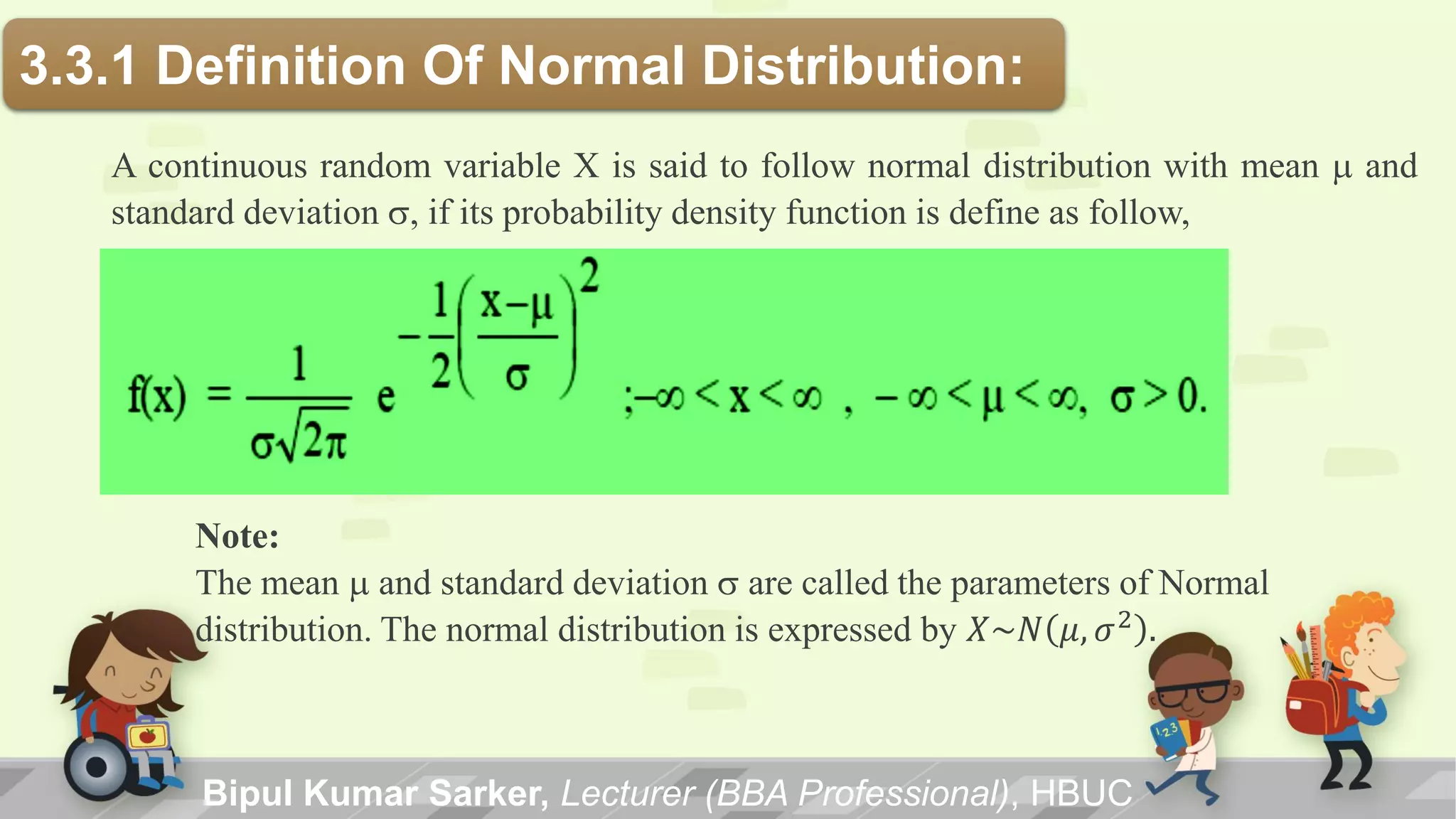
Definition of normal distribution with parameters: mean (m) and standard deviation (s). Notation: X~N(μ,σ²).
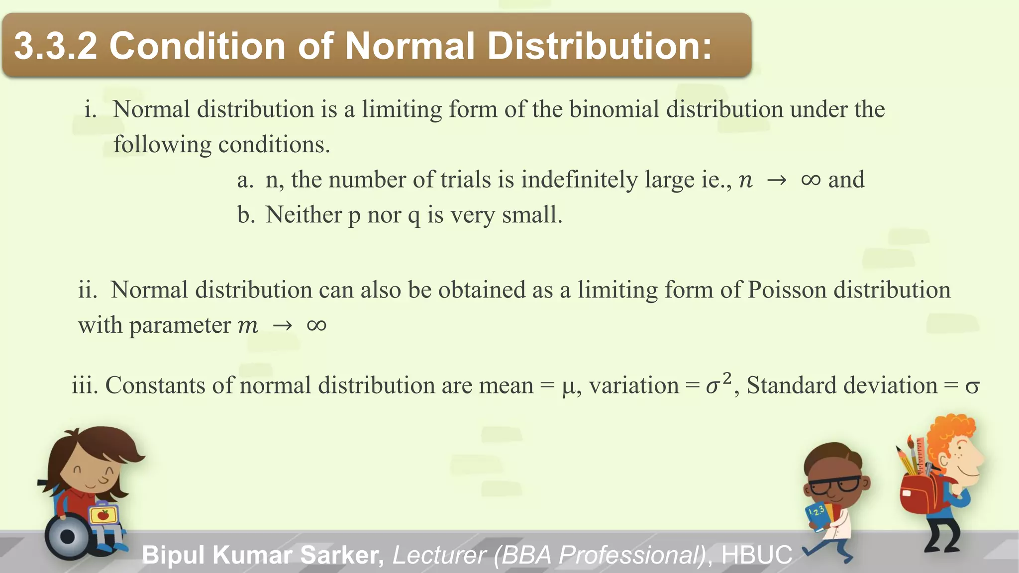
Conditions for normal distribution including limiting case of binomial and Poisson distributions.
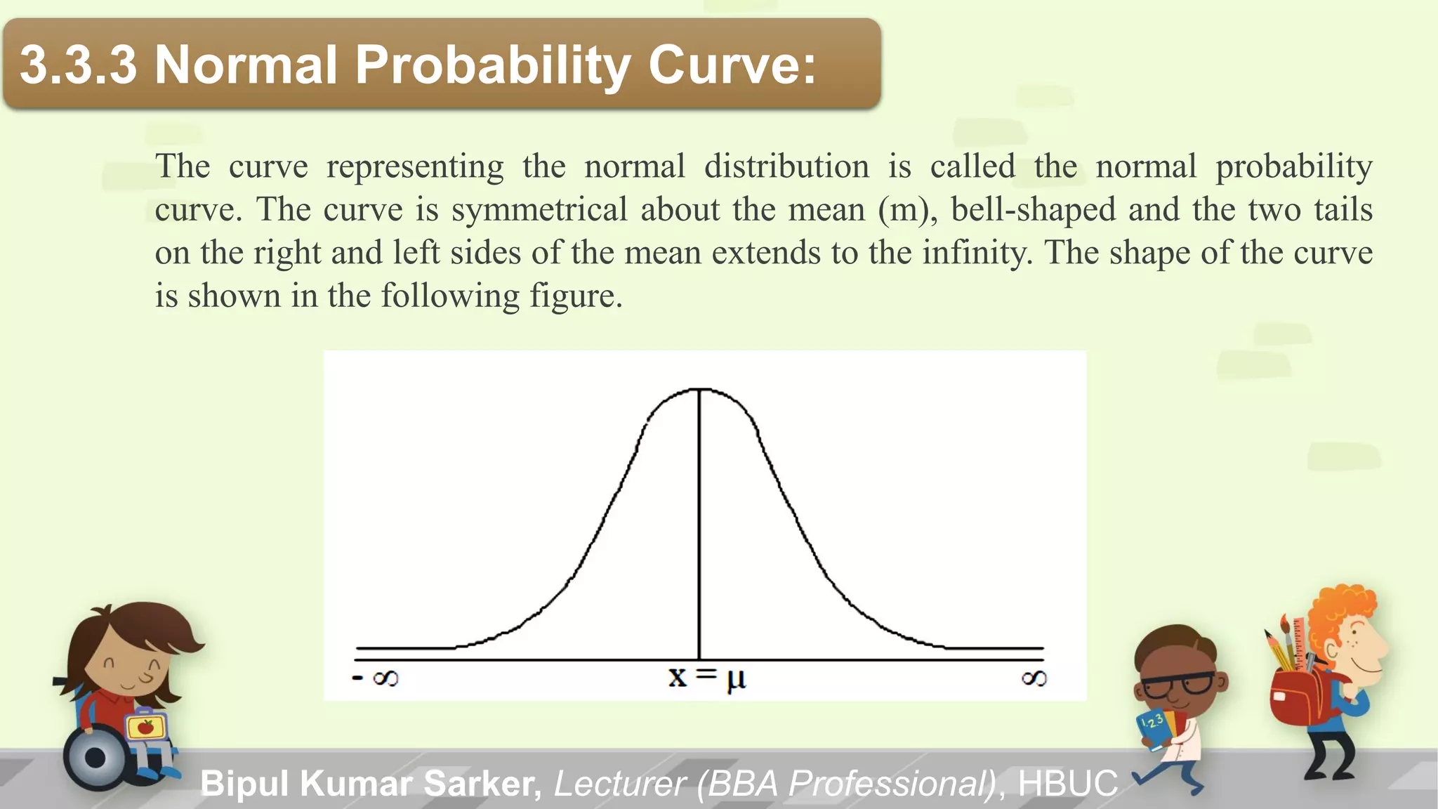
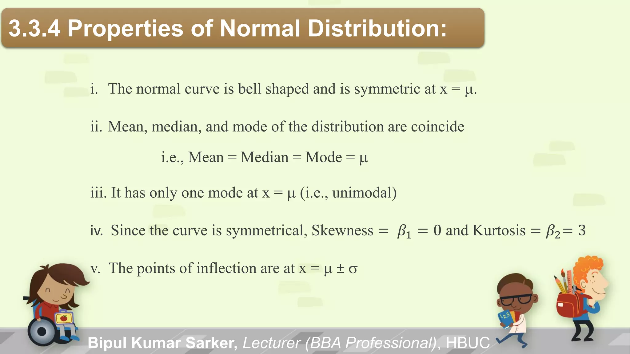
Characteristics of the normal probability curve: symmetrical around mean, bell-shaped, extends to infinity.
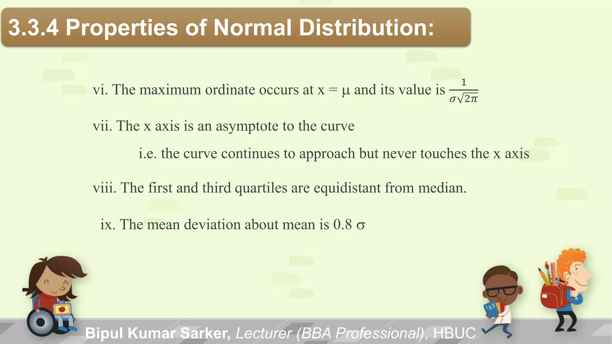
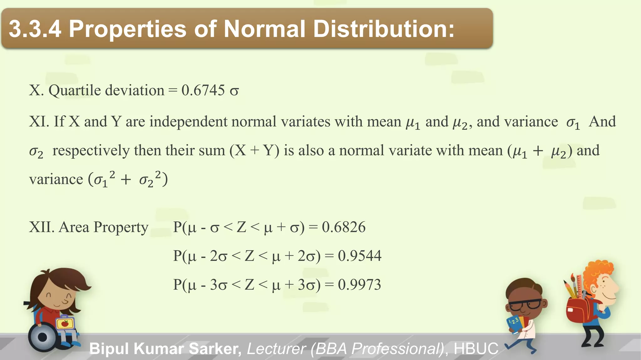
Key properties: symmetric, unimodal, mean=median=mode, skewness=0, inflection points, quartile properties.
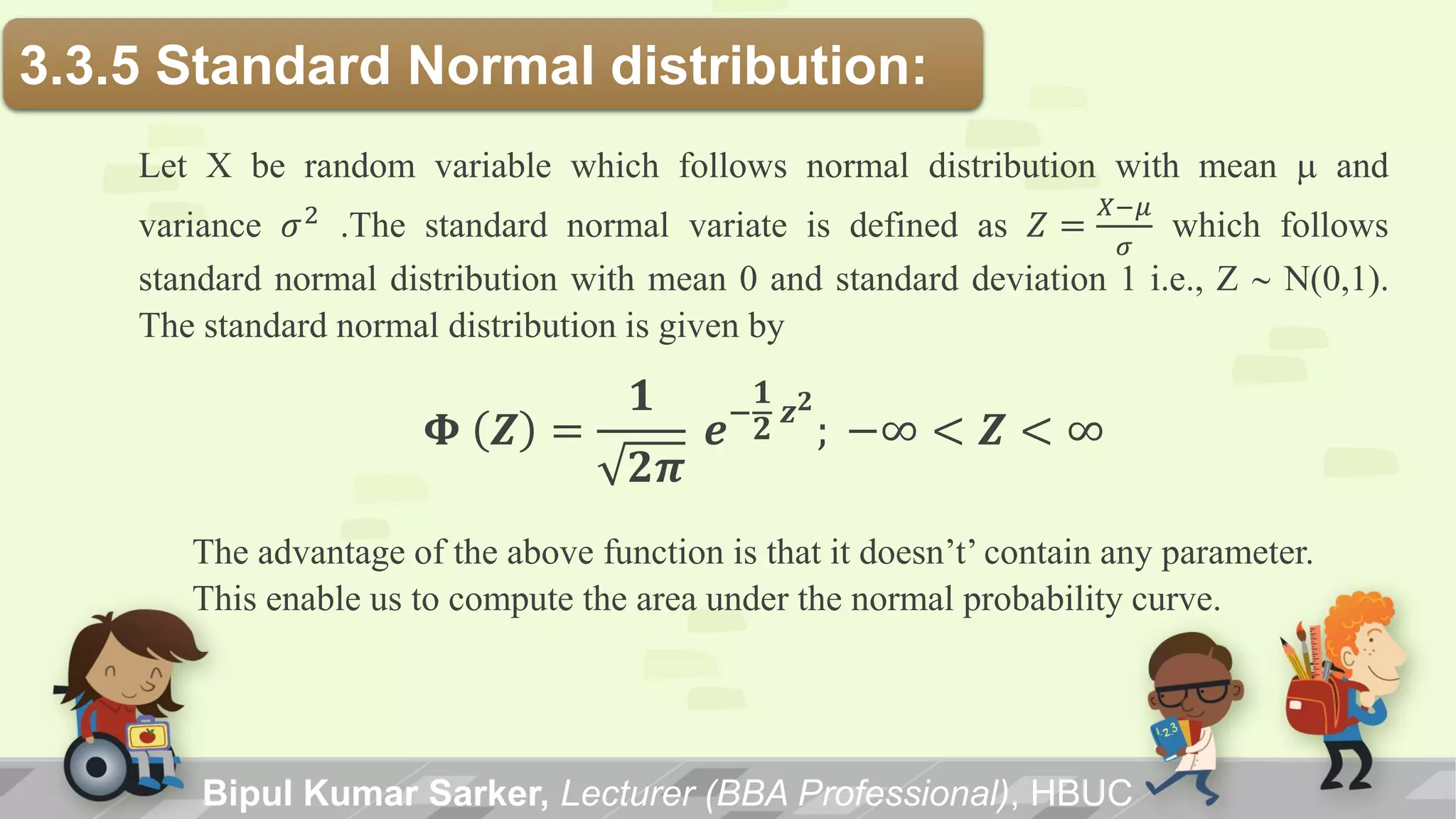
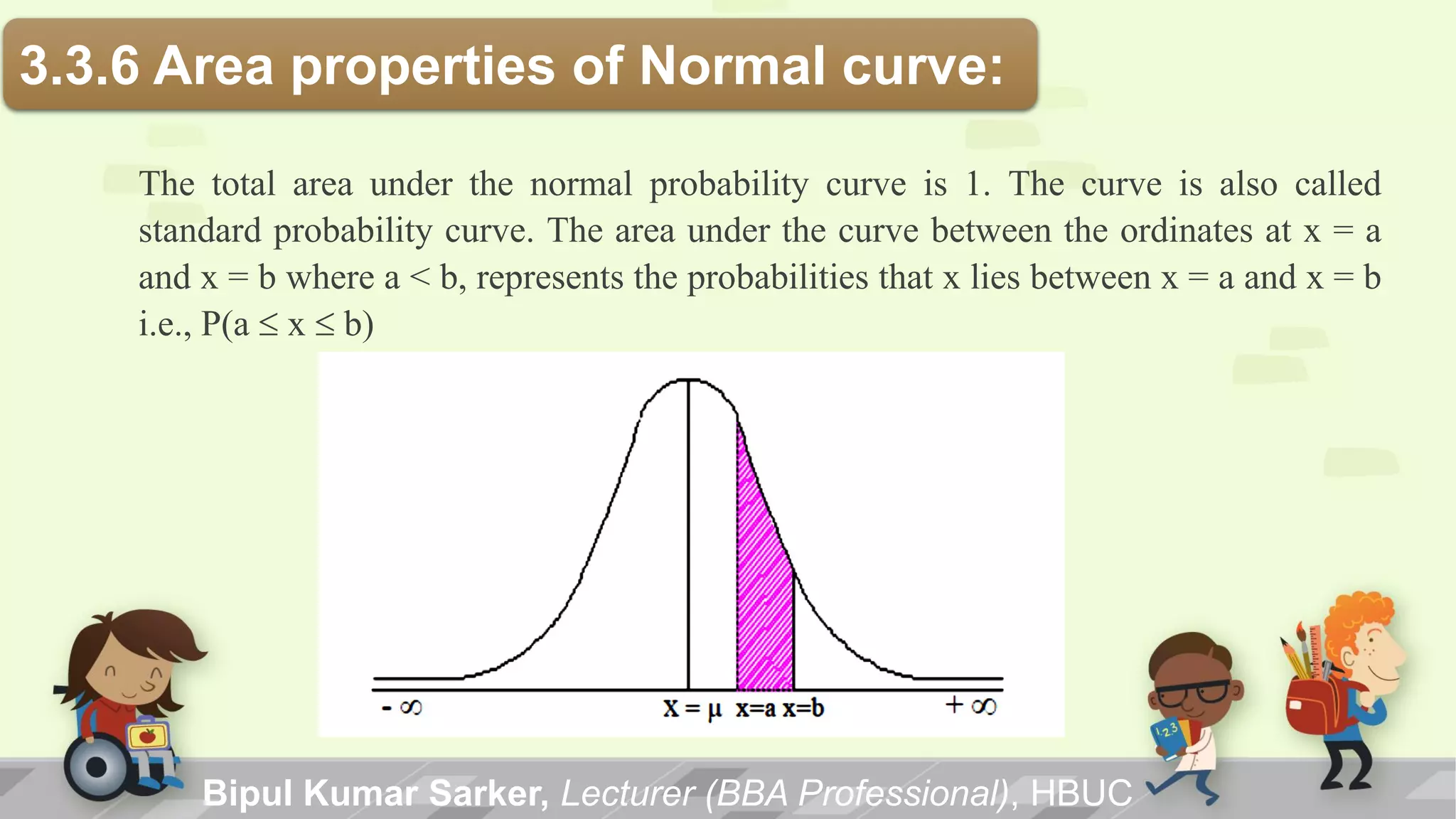
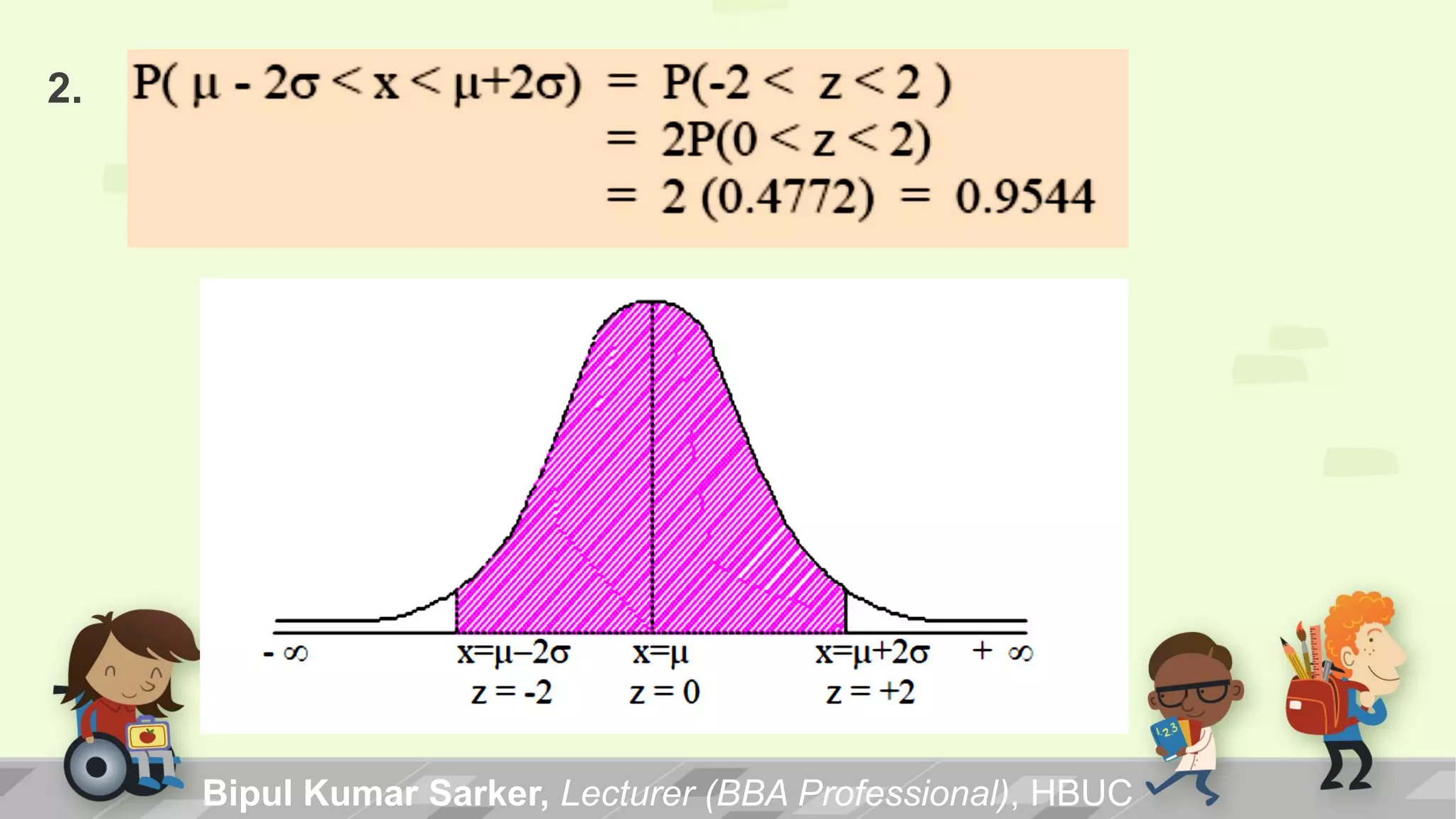
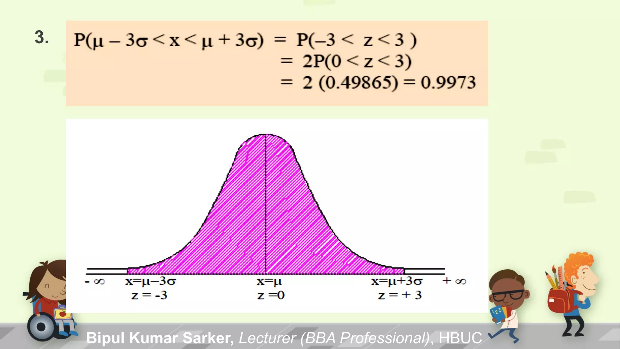
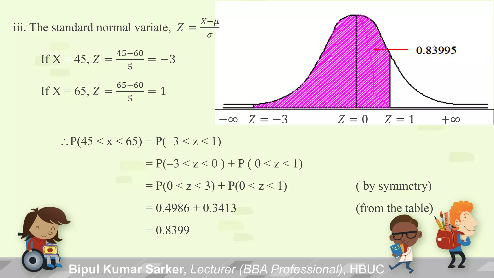
Standard normal distribution defined with Z-score formula, area properties under the normal curve.
How to standardize a random variable using Z-score for probability calculations.
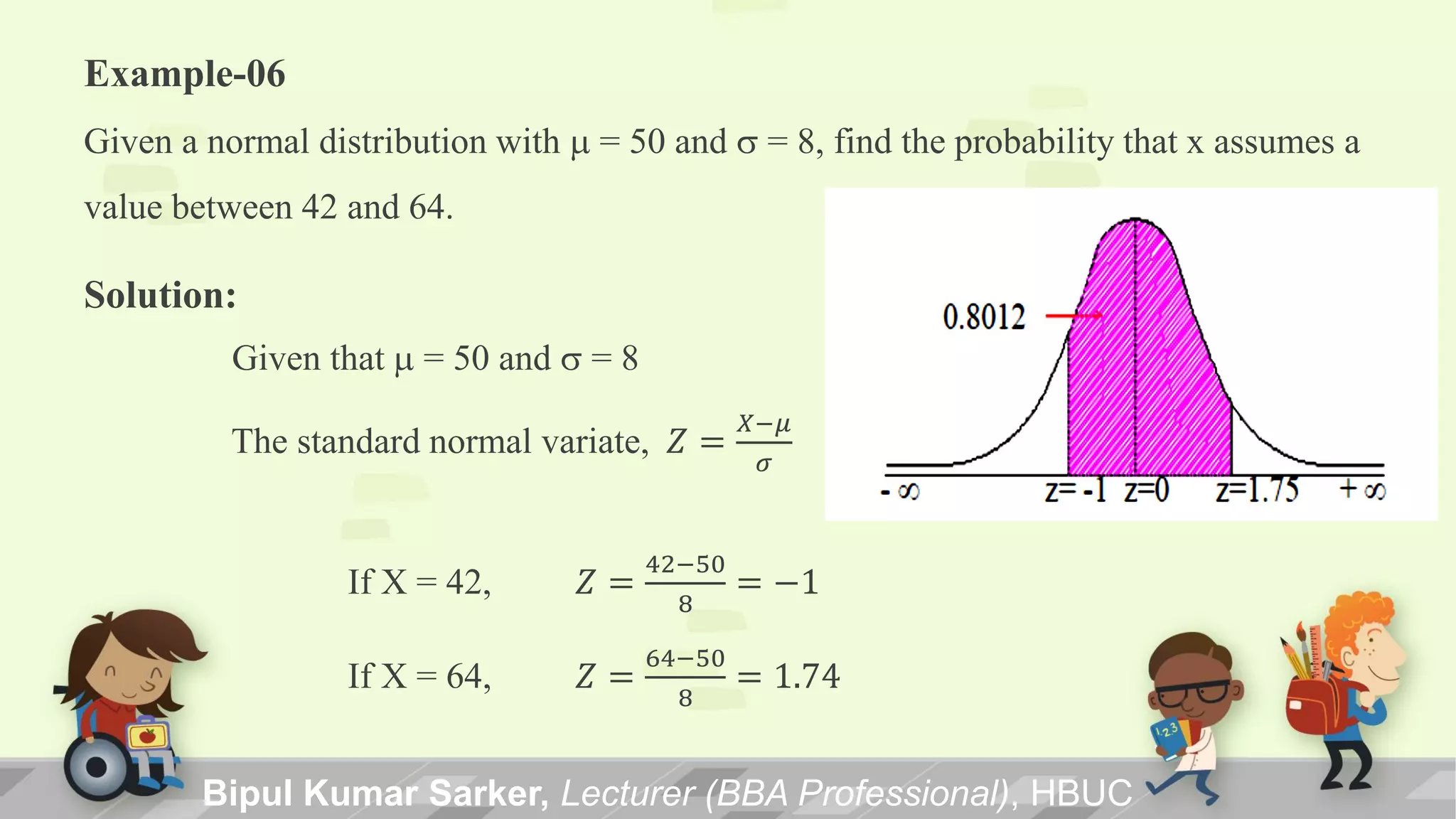
Example showing probability for a normal random variable within specific intervals.
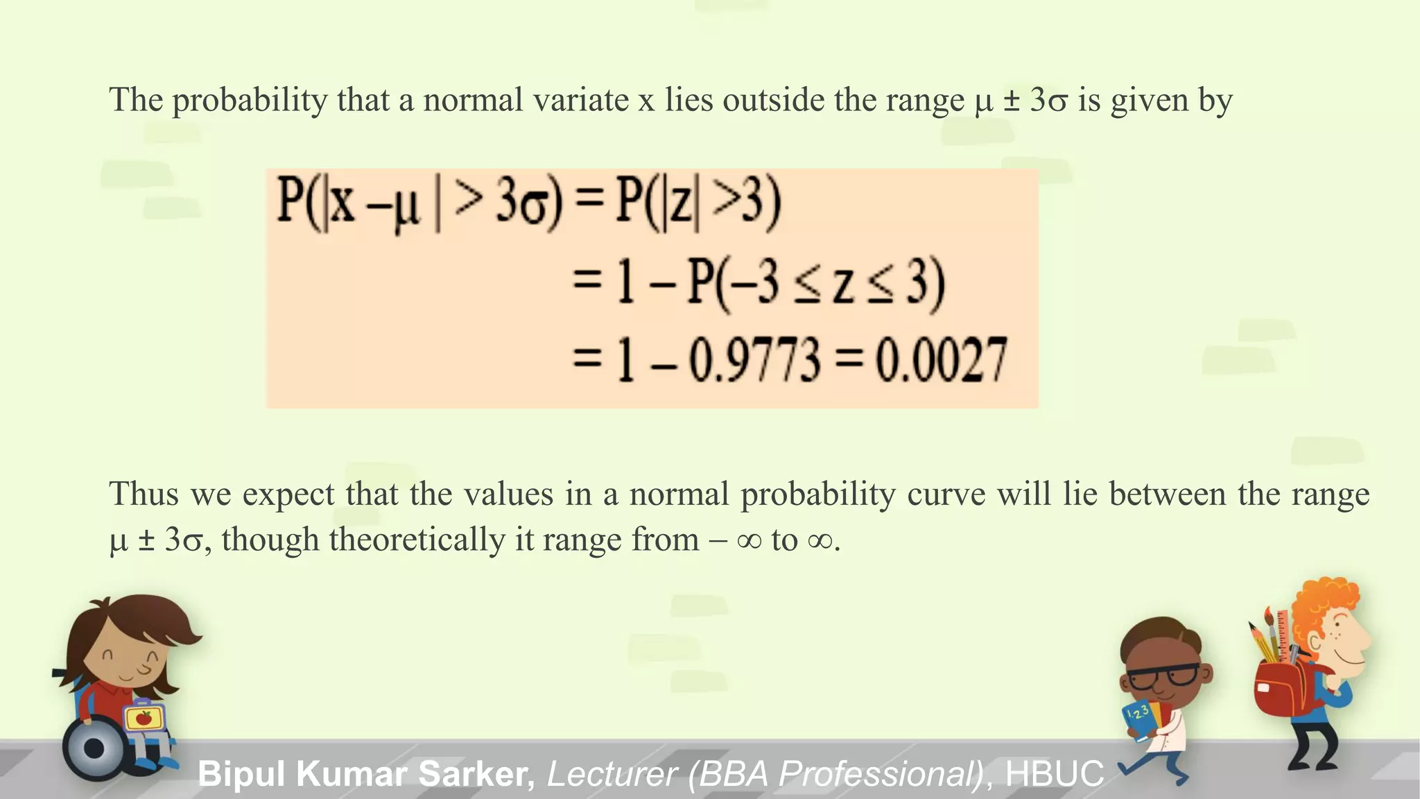
Insights into the expectation of normal variate values within range m ± 3s.
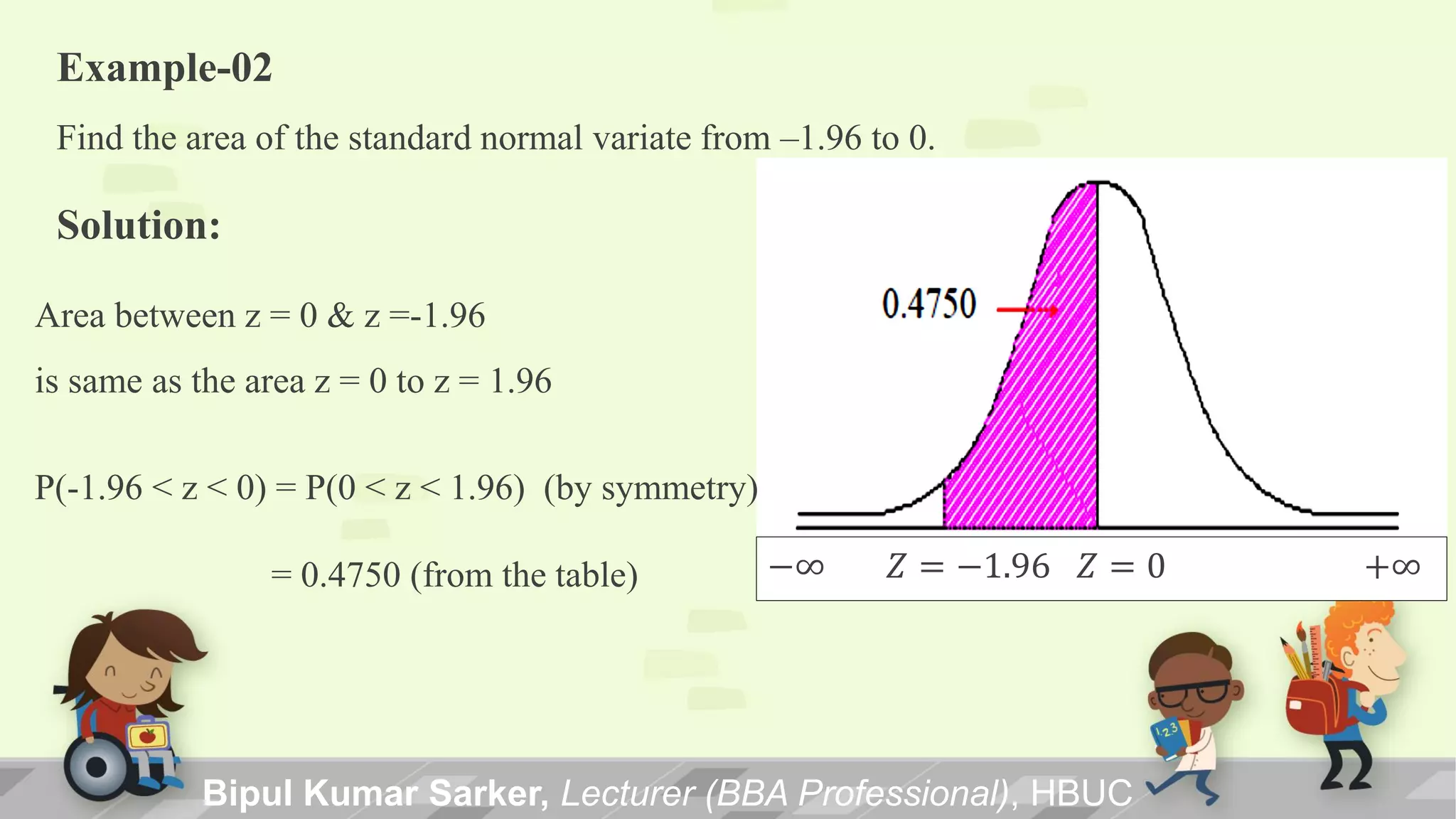
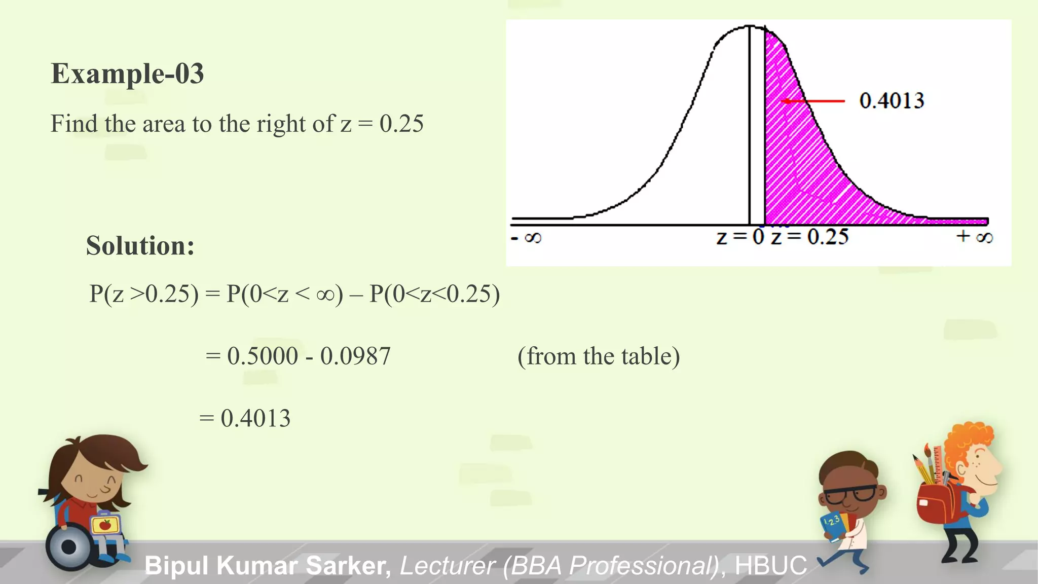
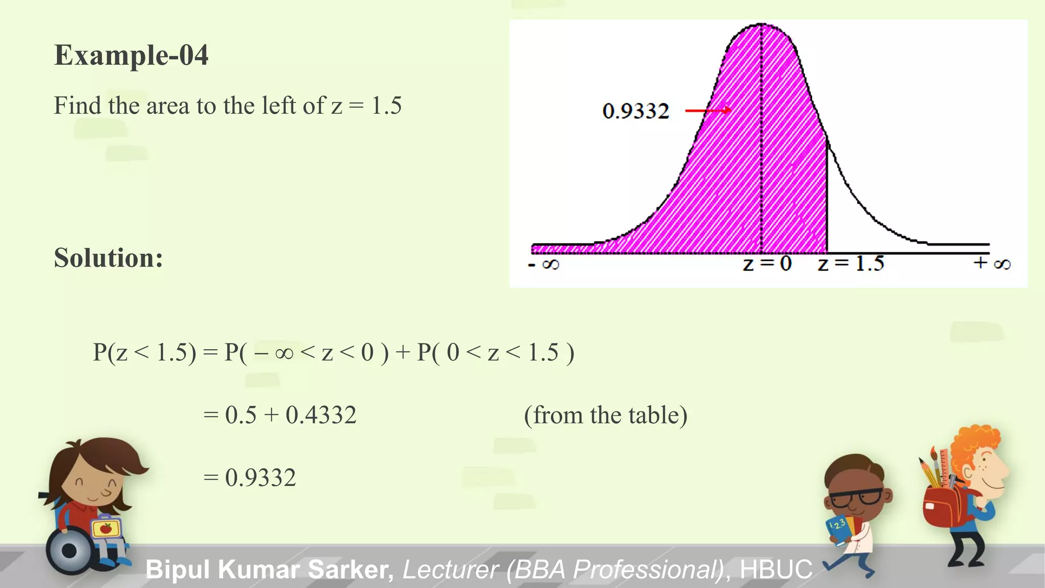
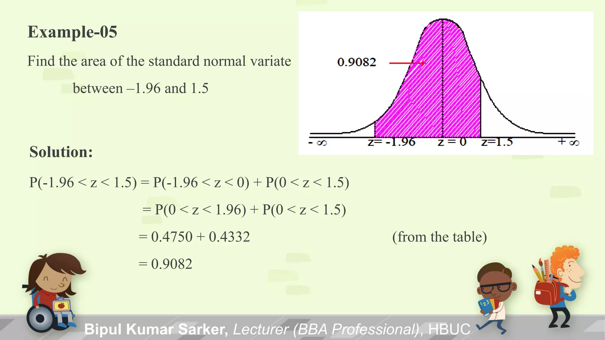
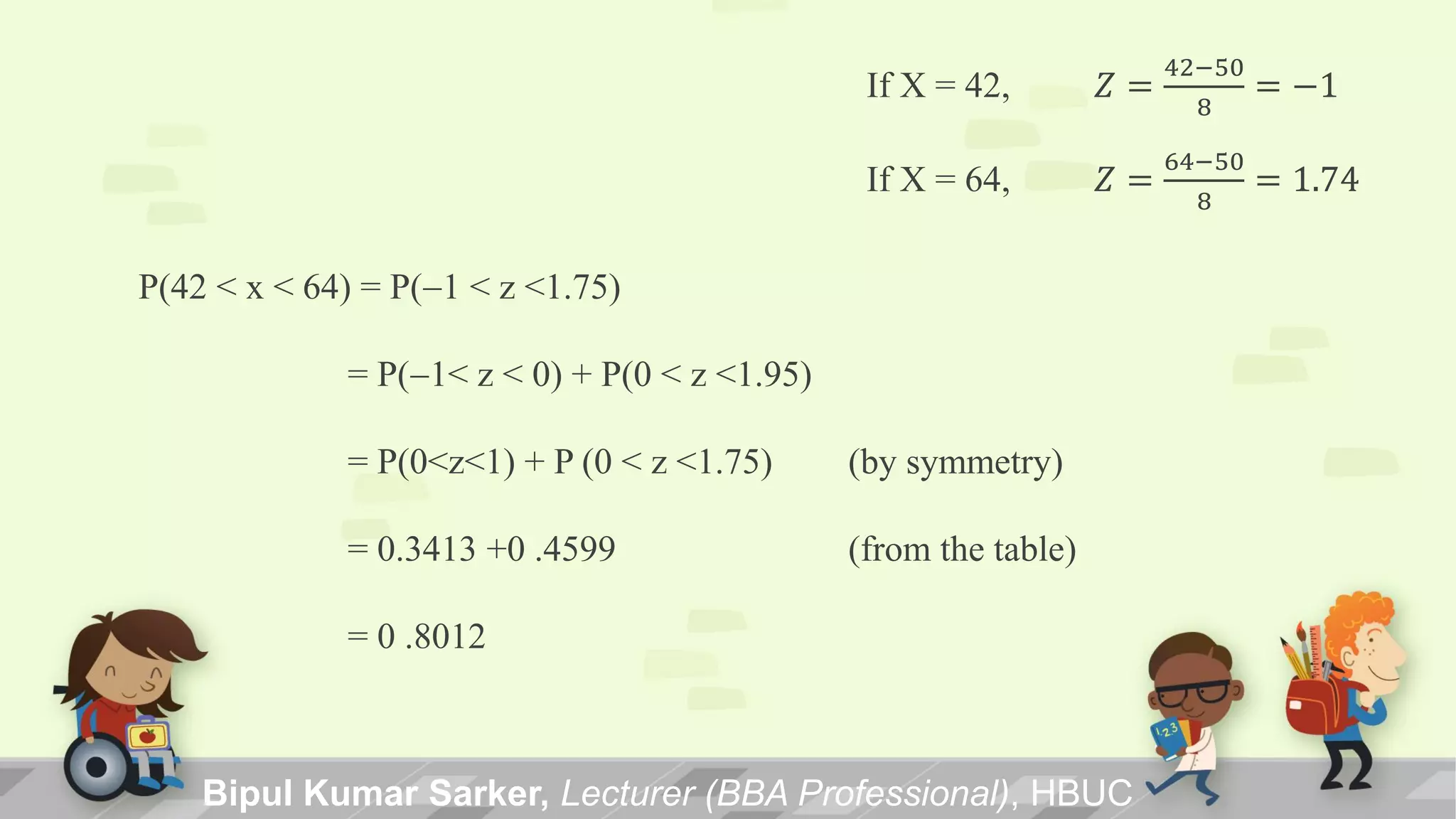
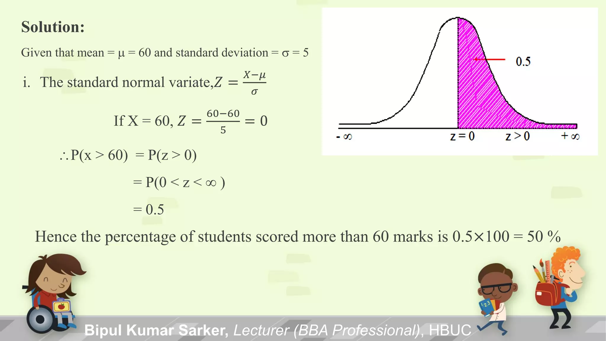
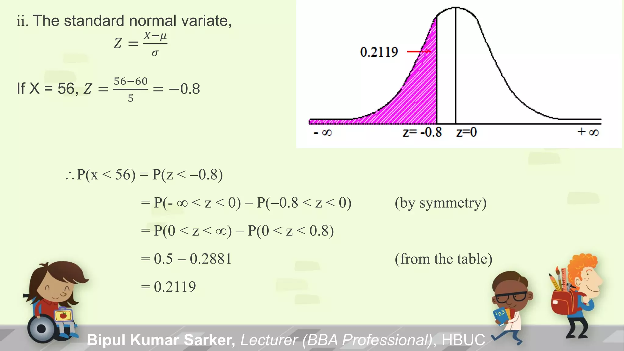
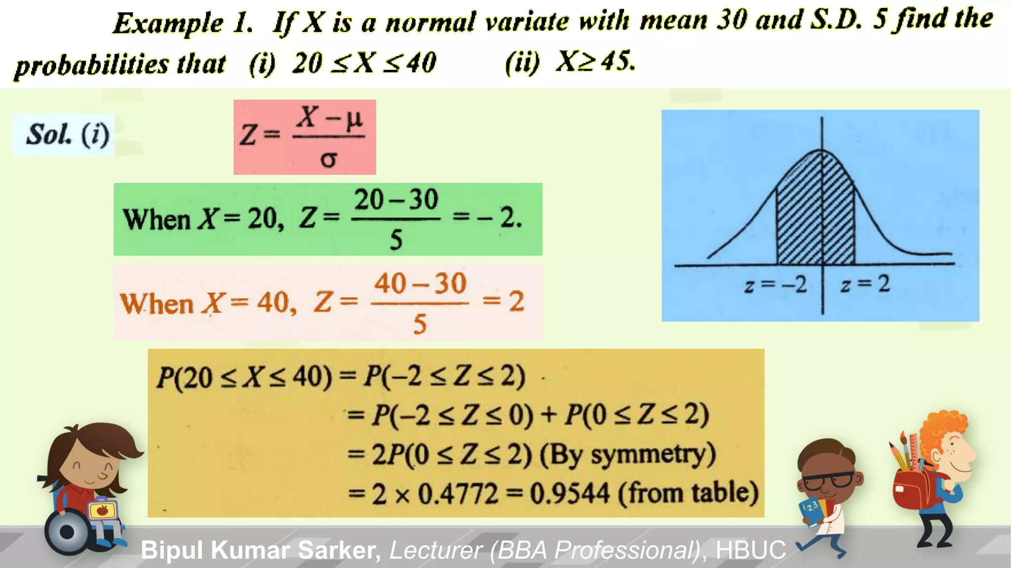
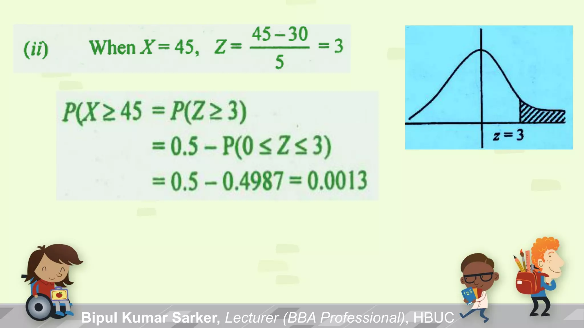
Multiple examples demonstrating Z-score calculations and areas/probabilities related to normal distribution.
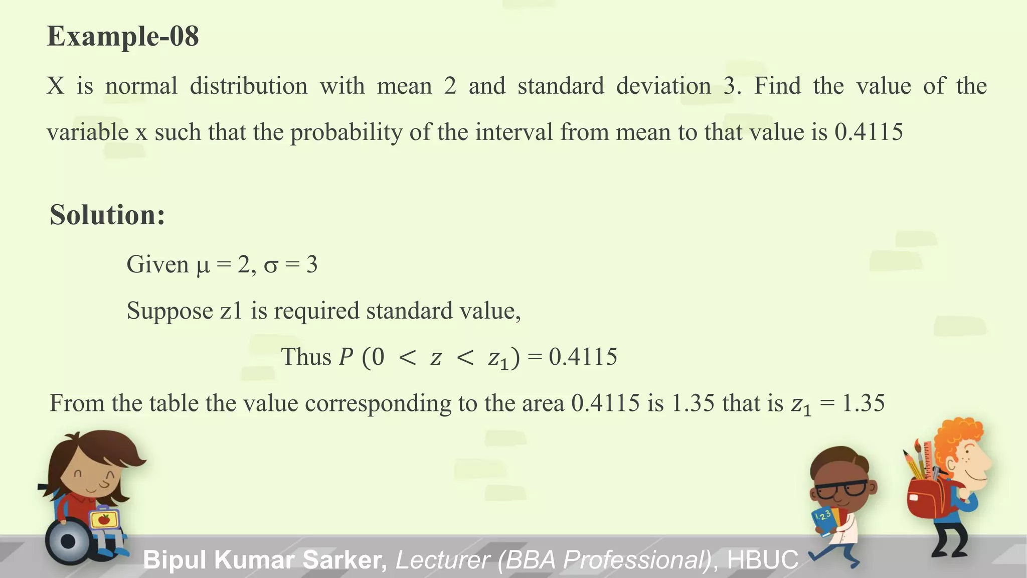
Final example illustrating how to determine variable value from normal distribution based on probability.


