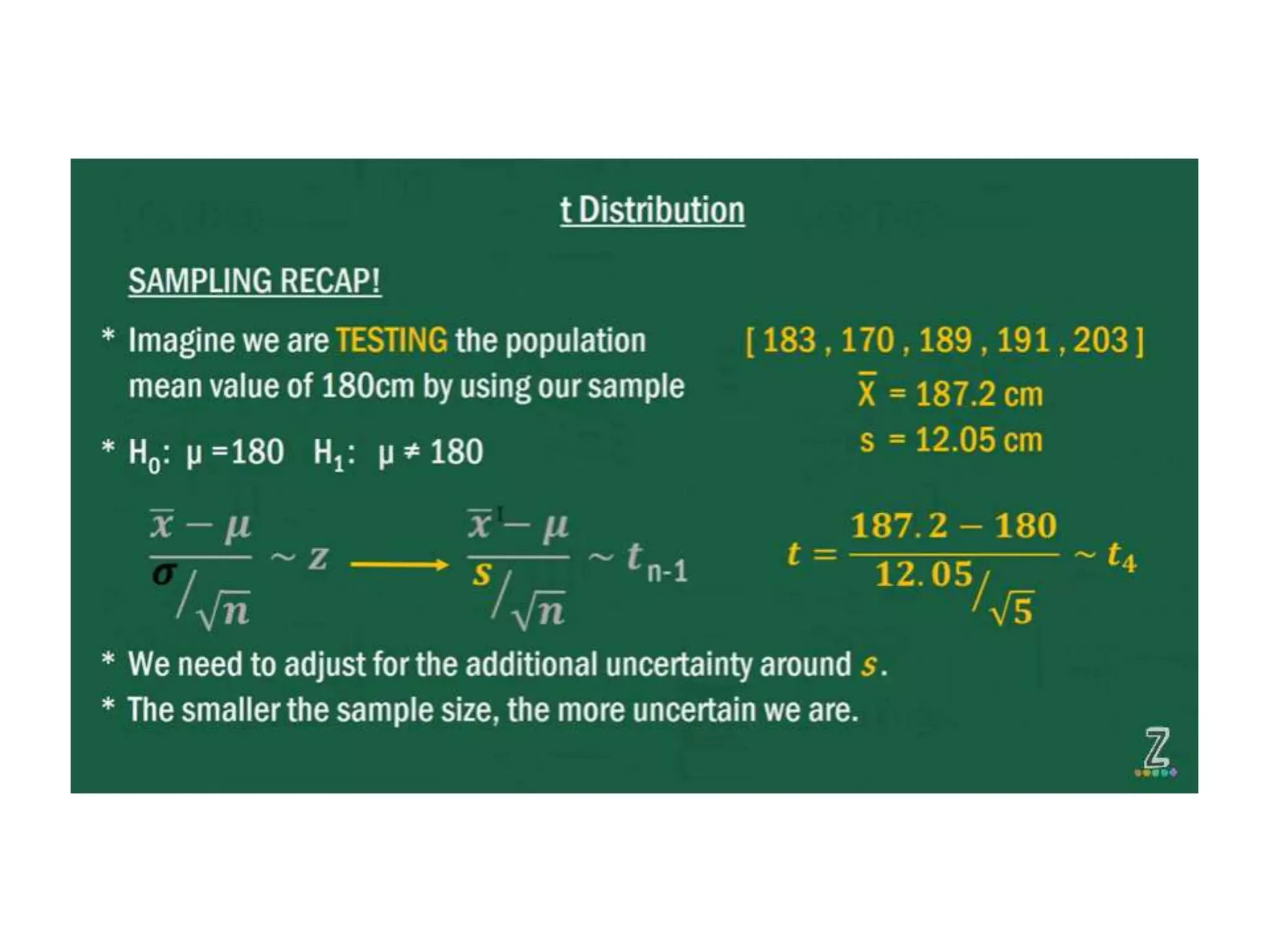
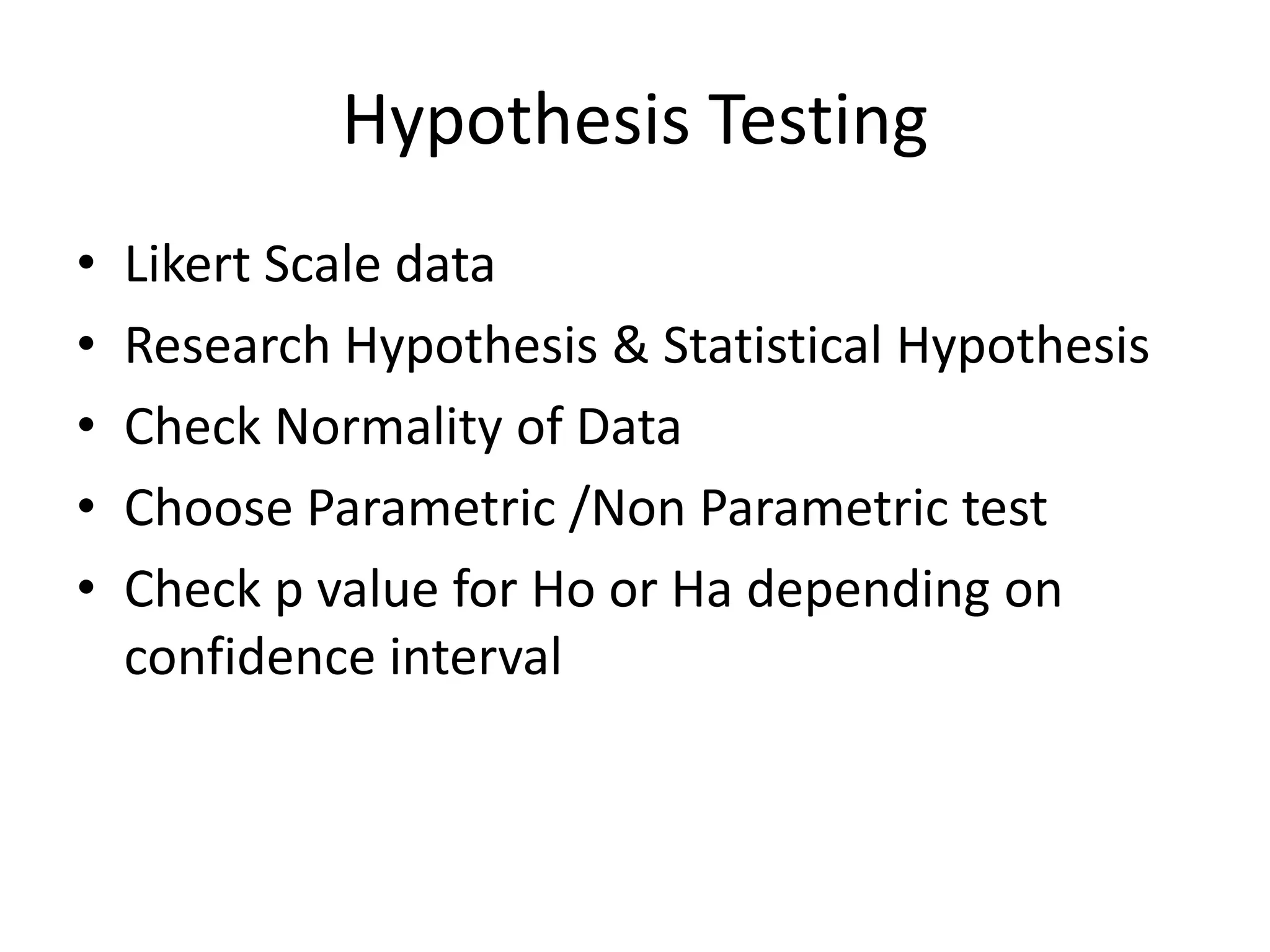
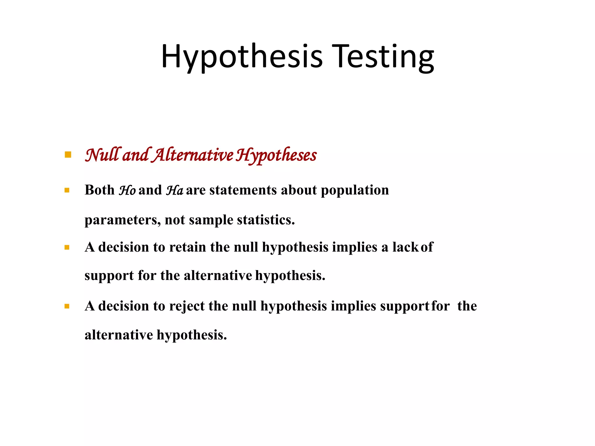
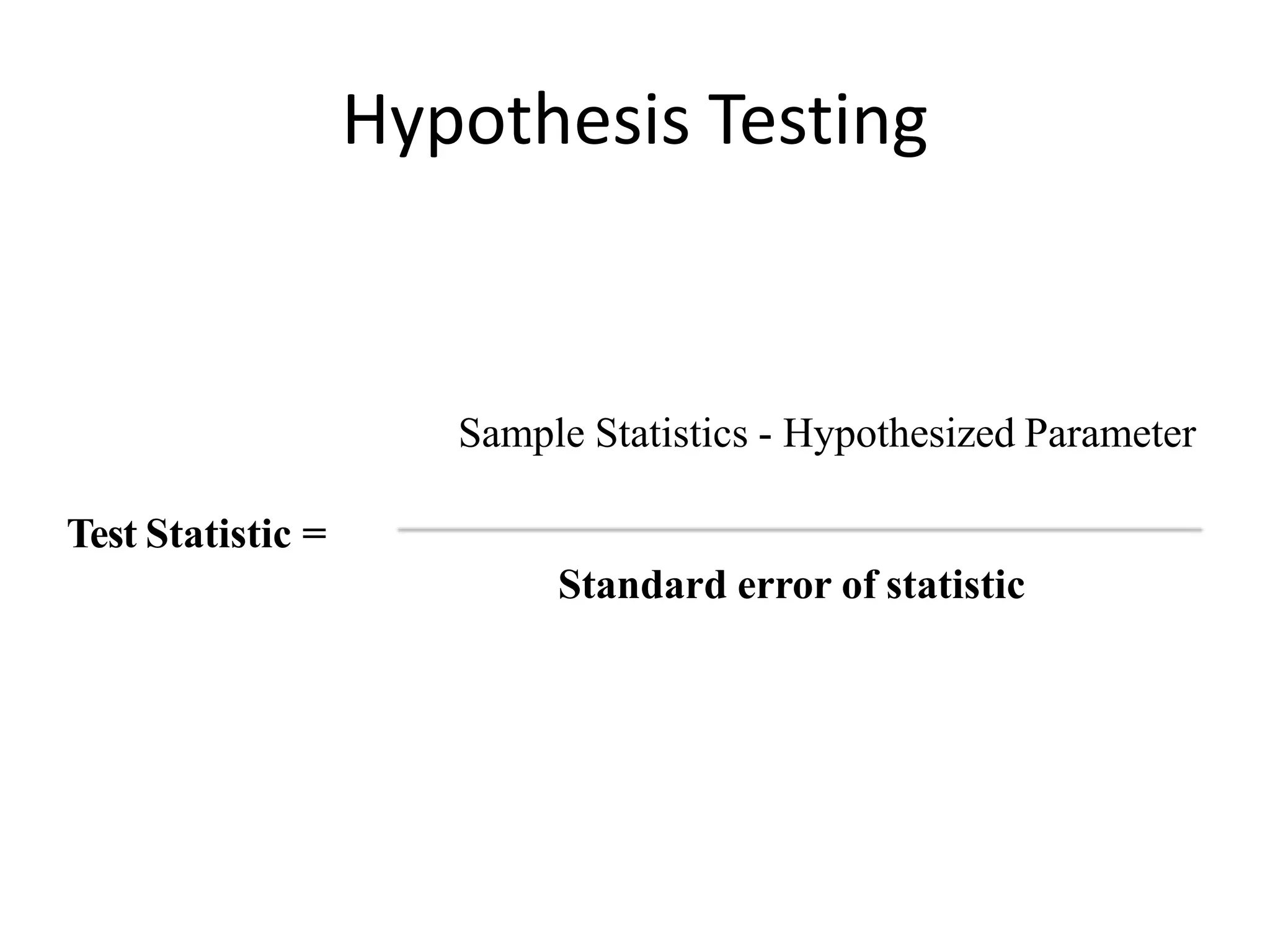
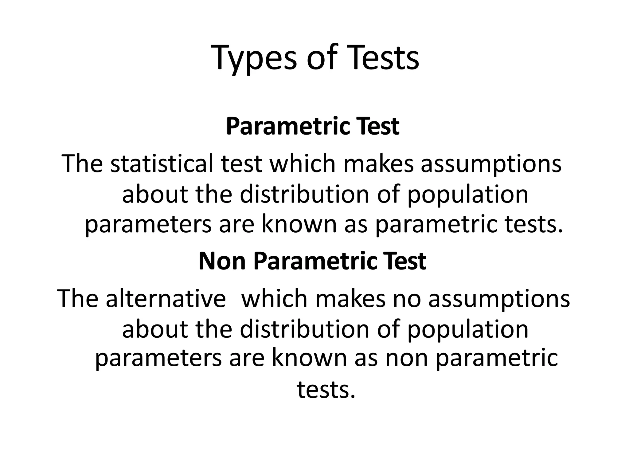
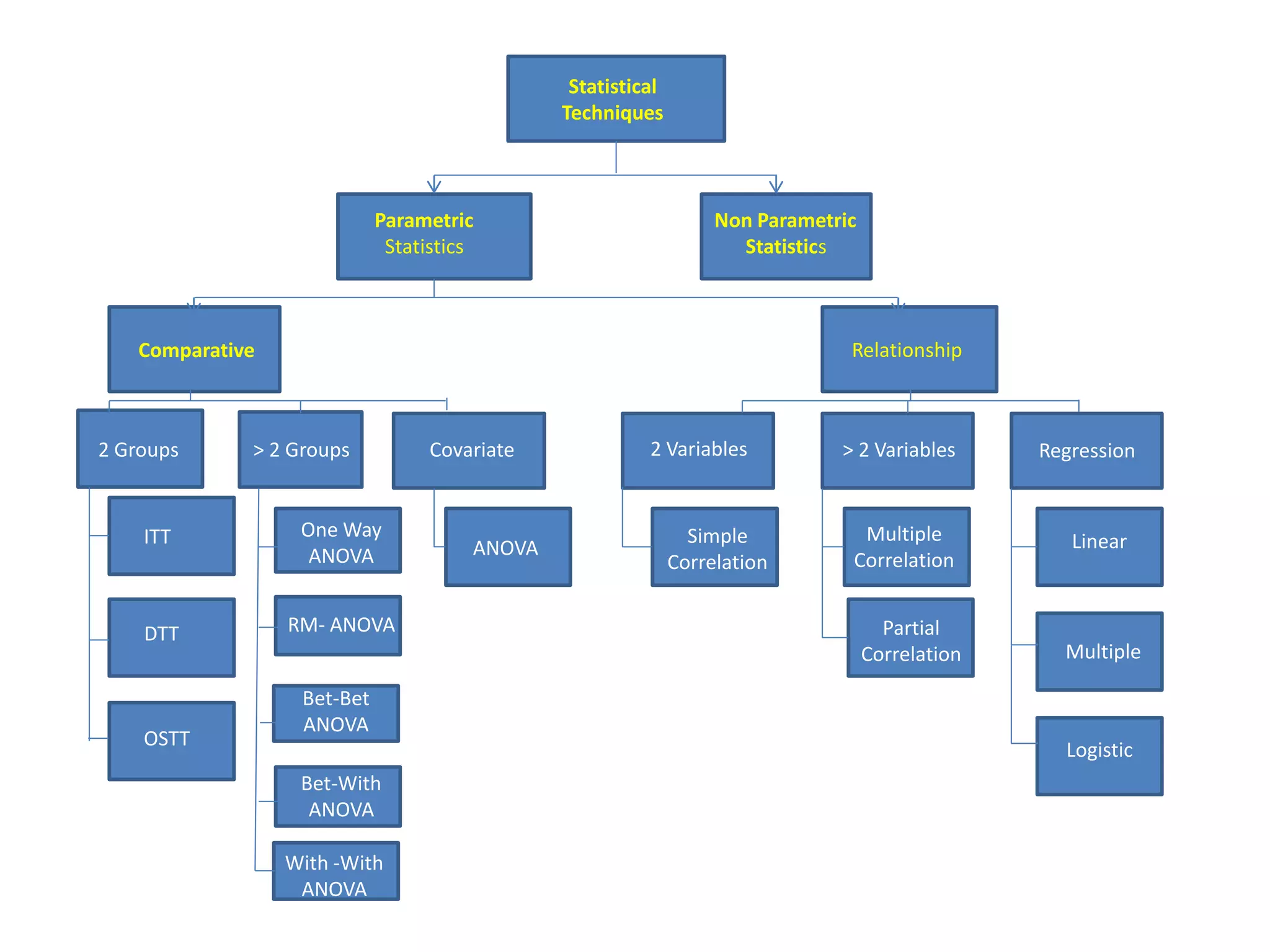
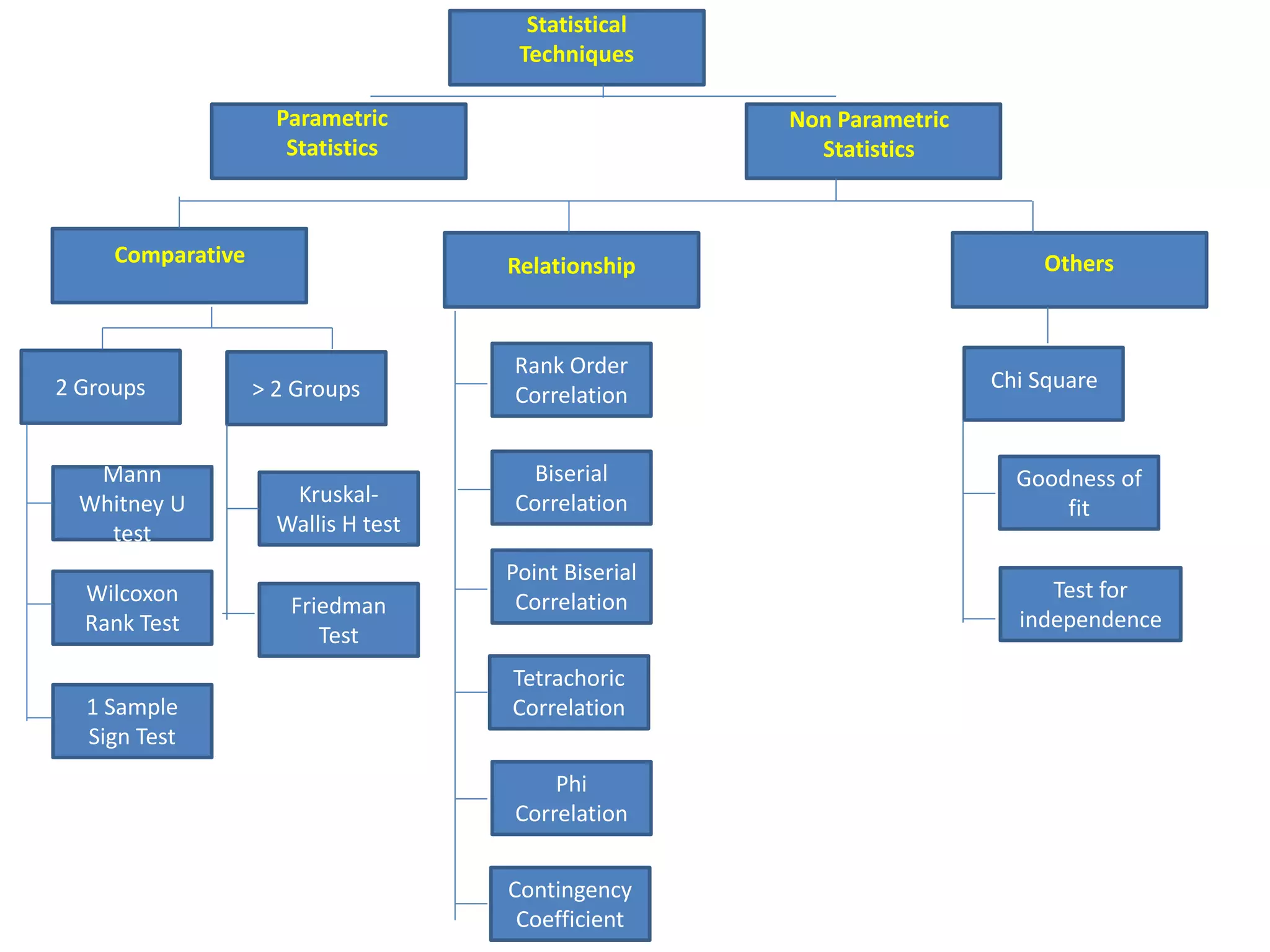
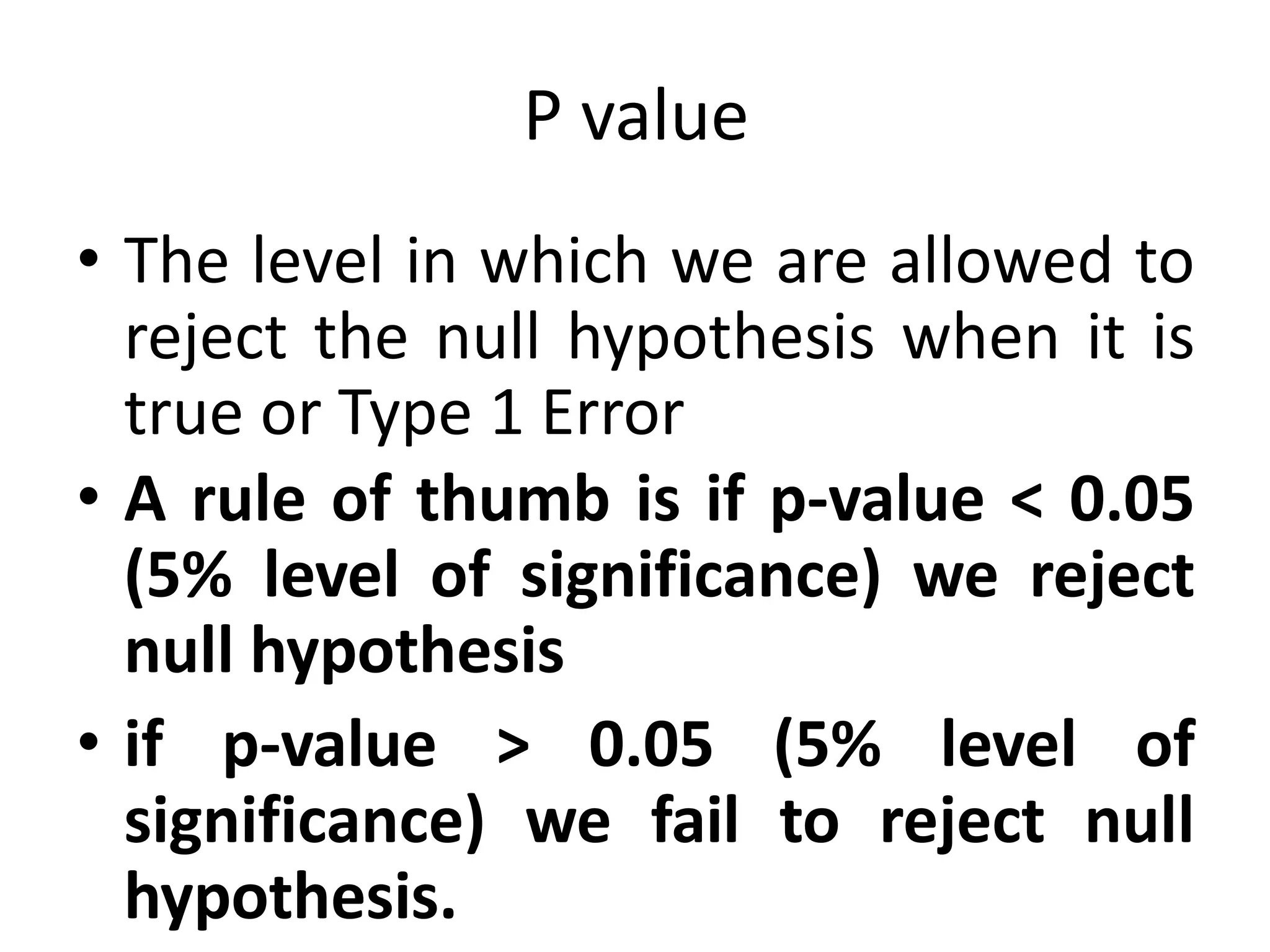
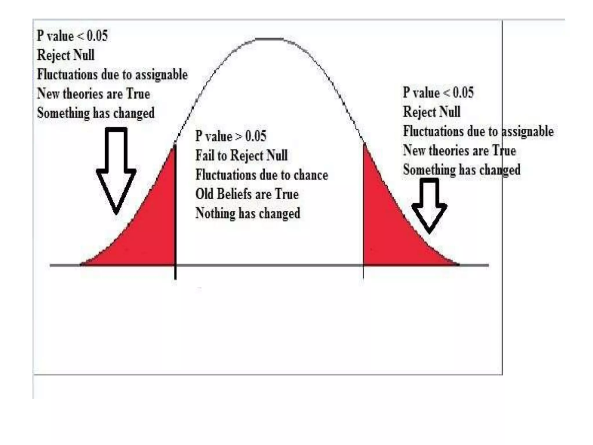
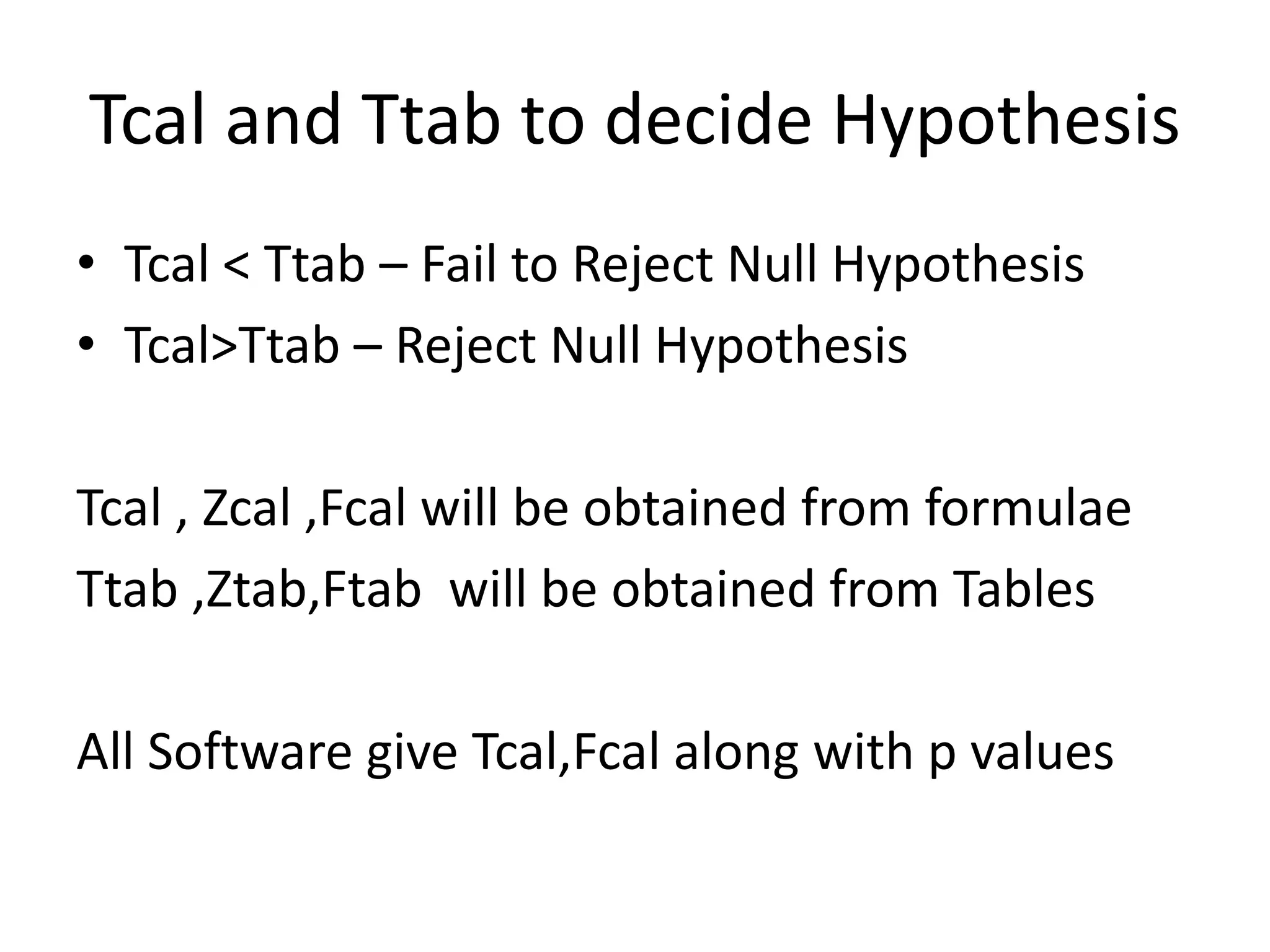
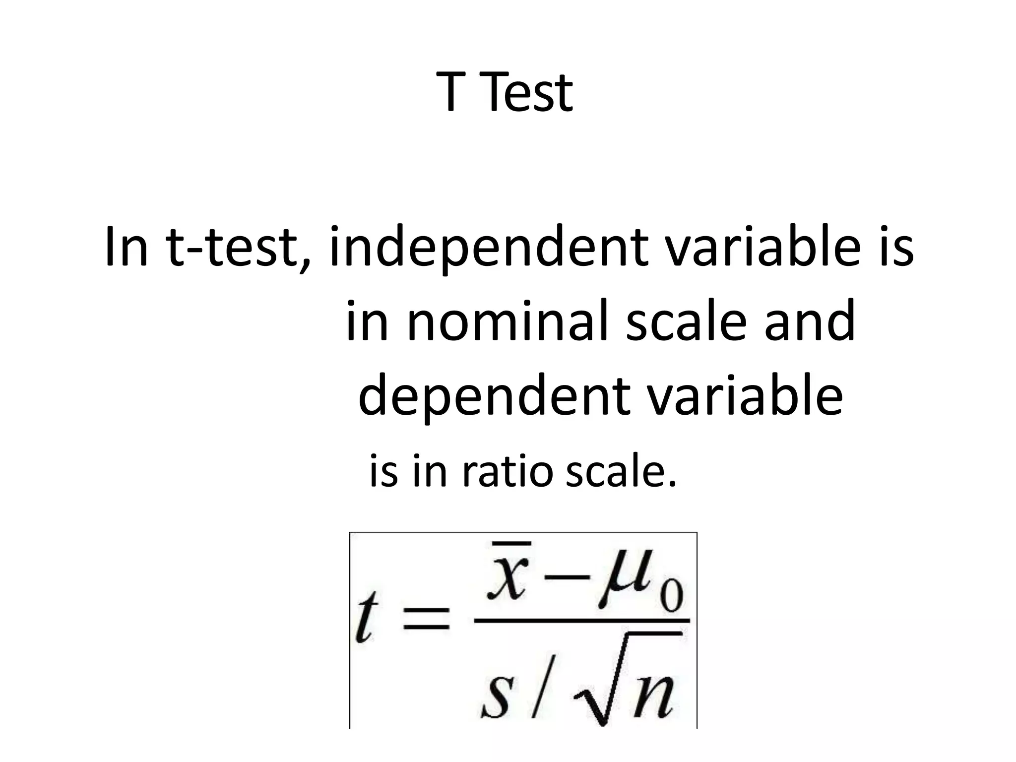
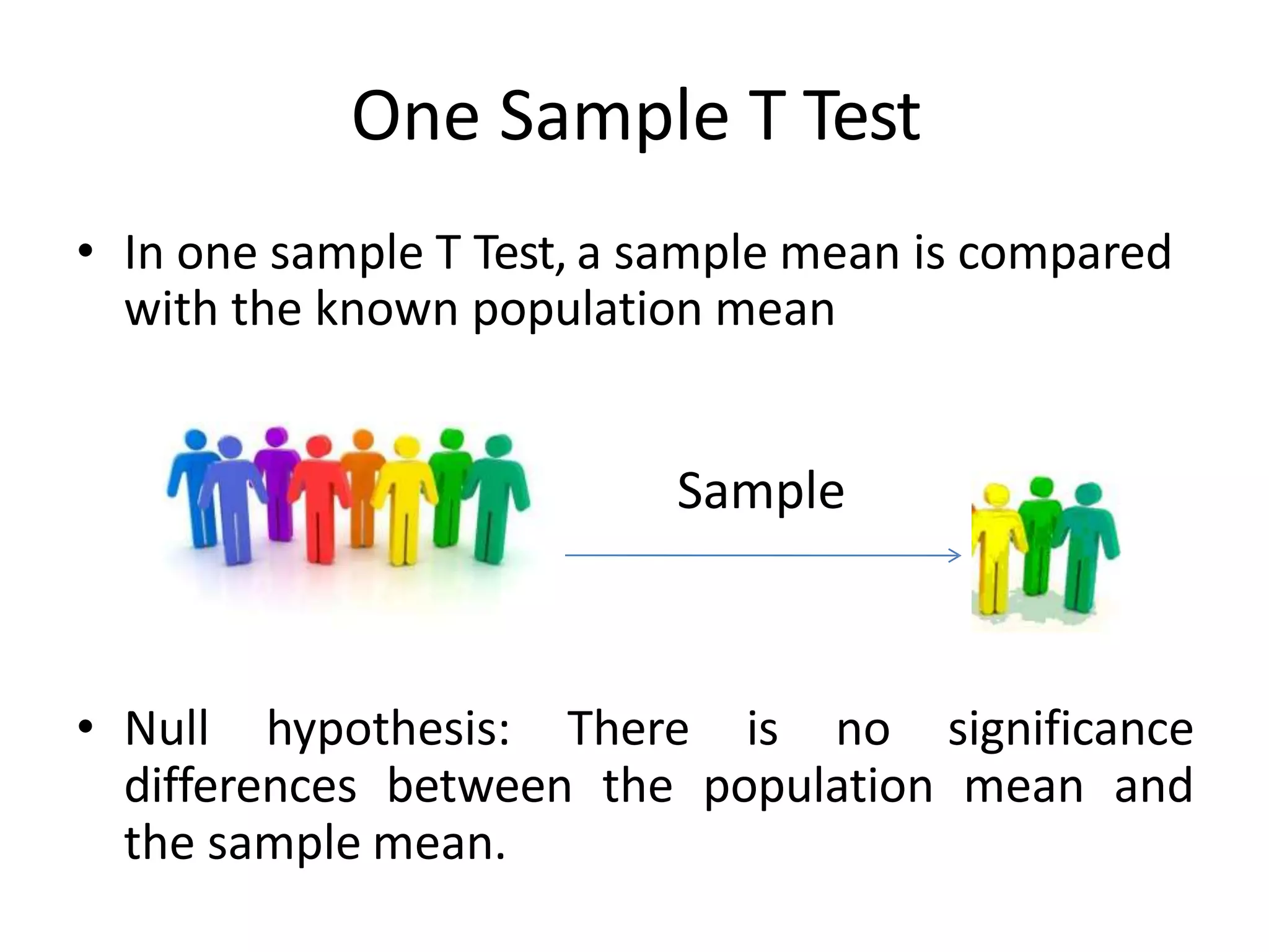
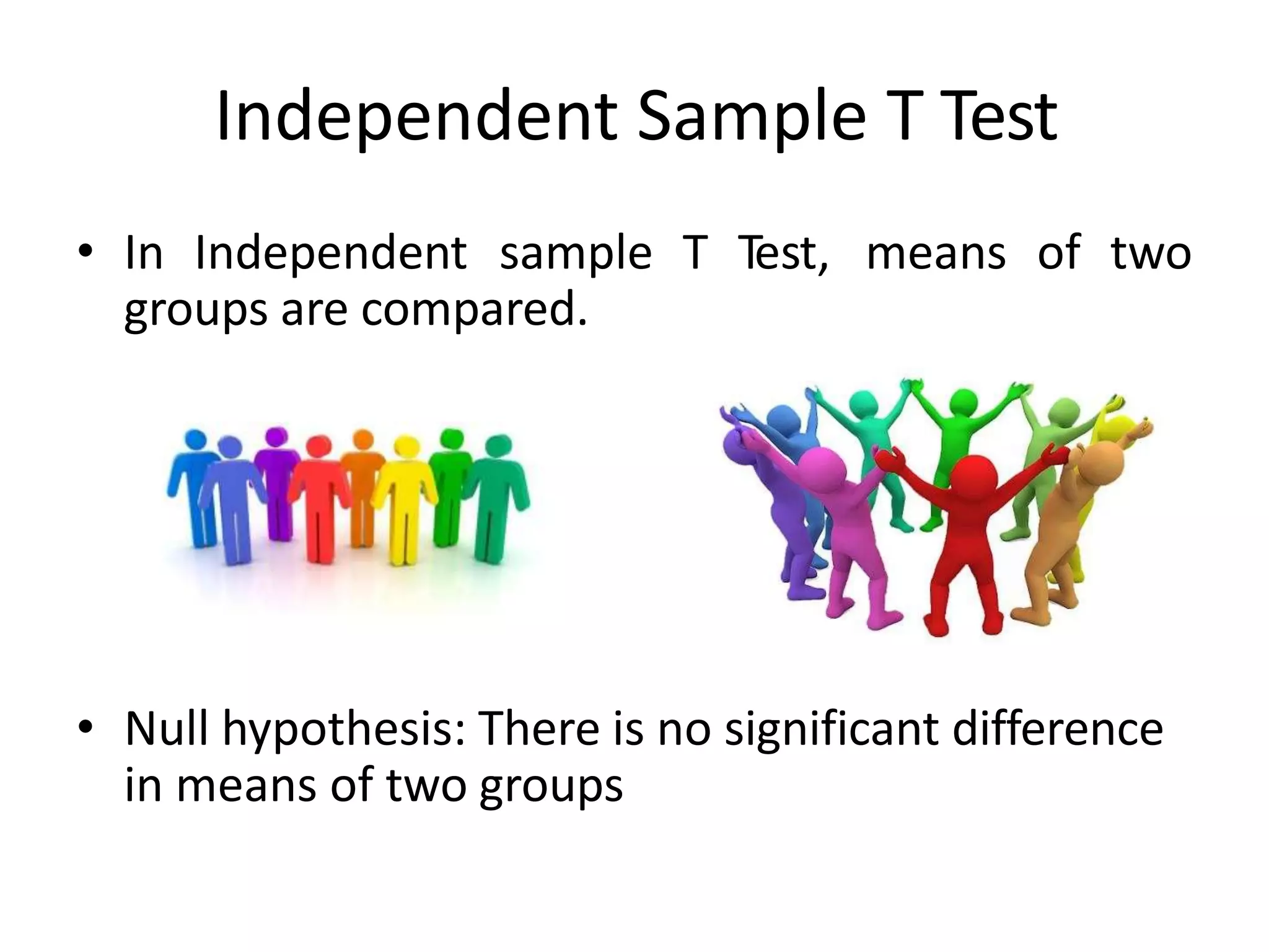
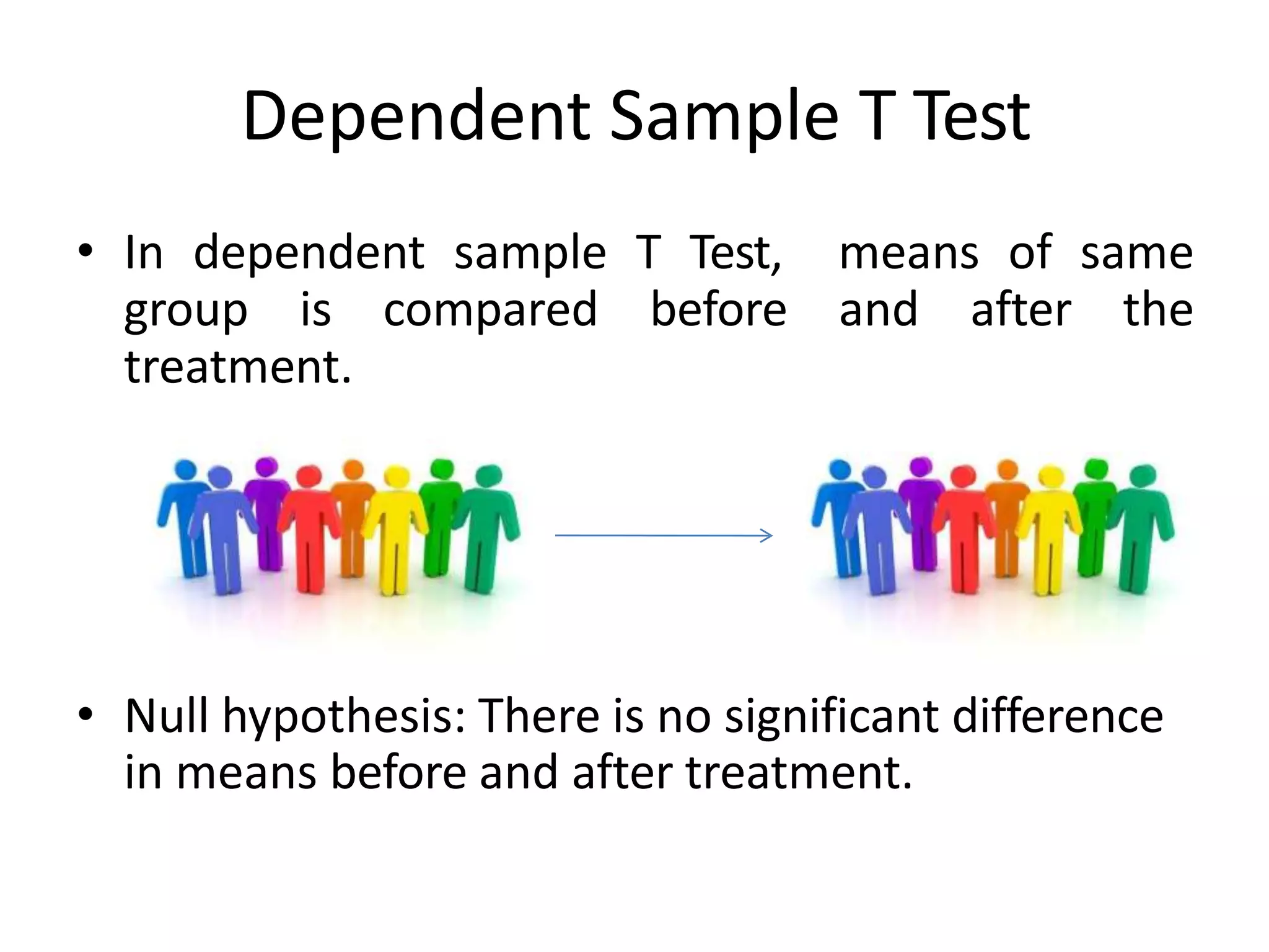
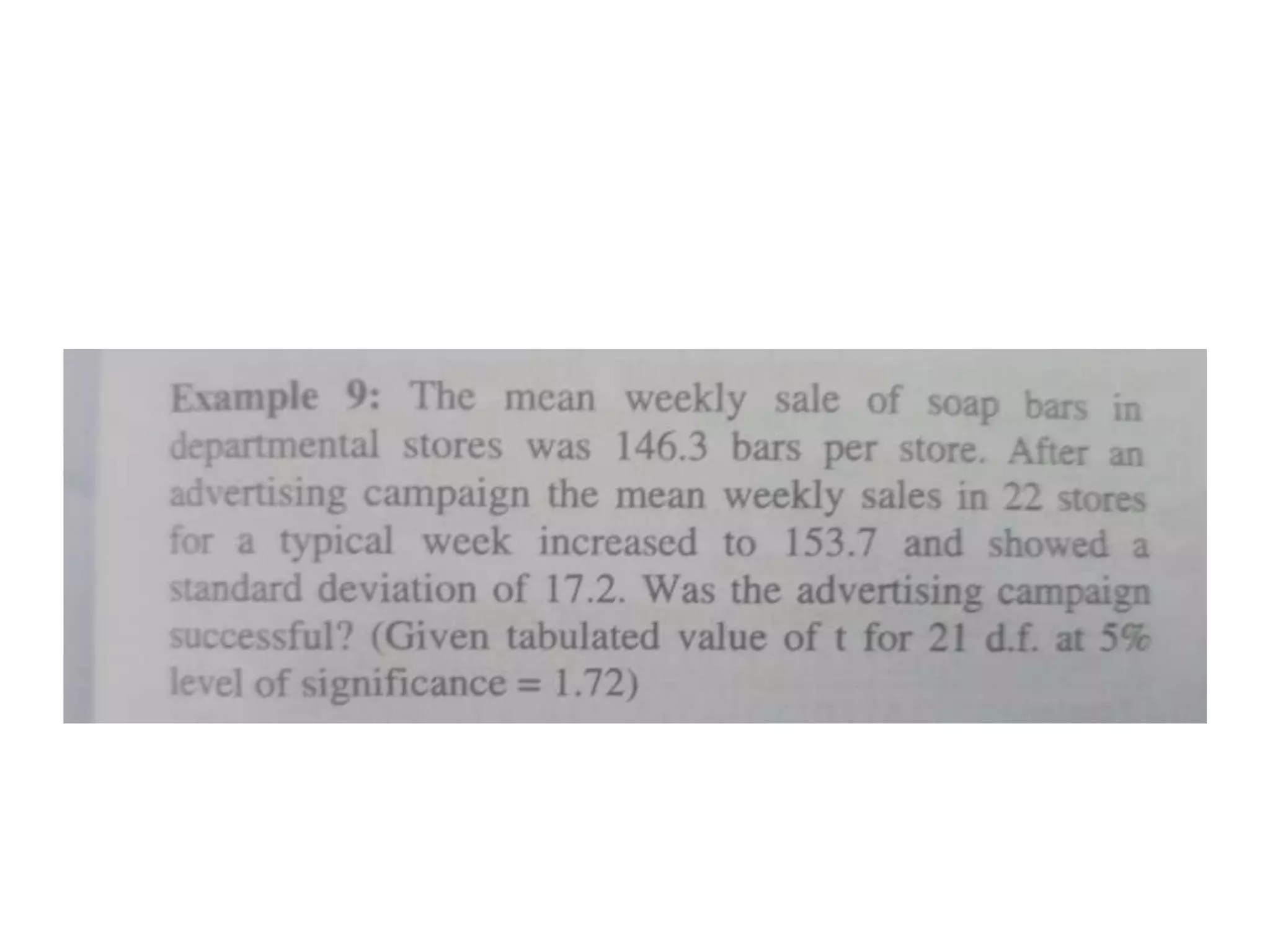
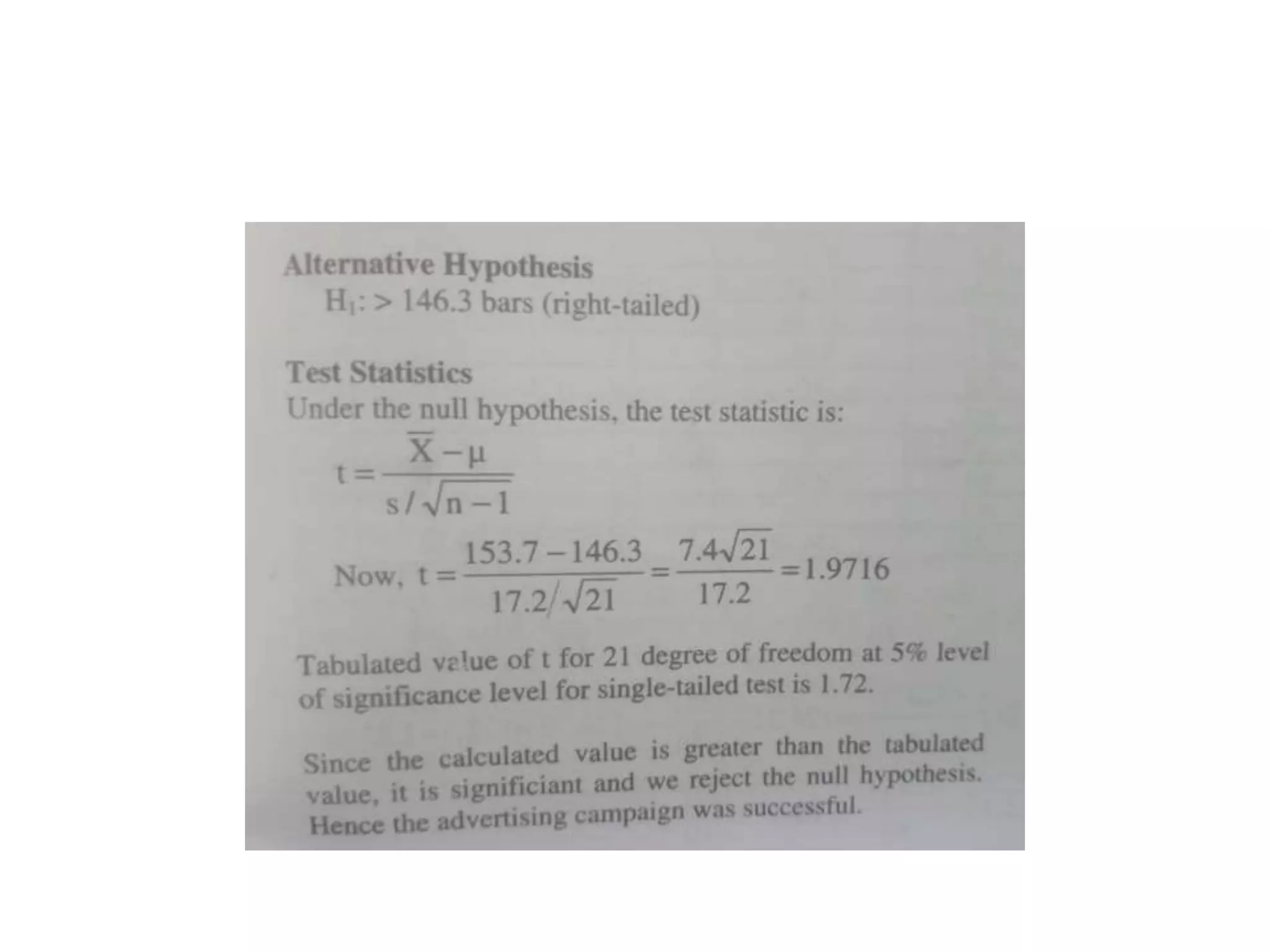
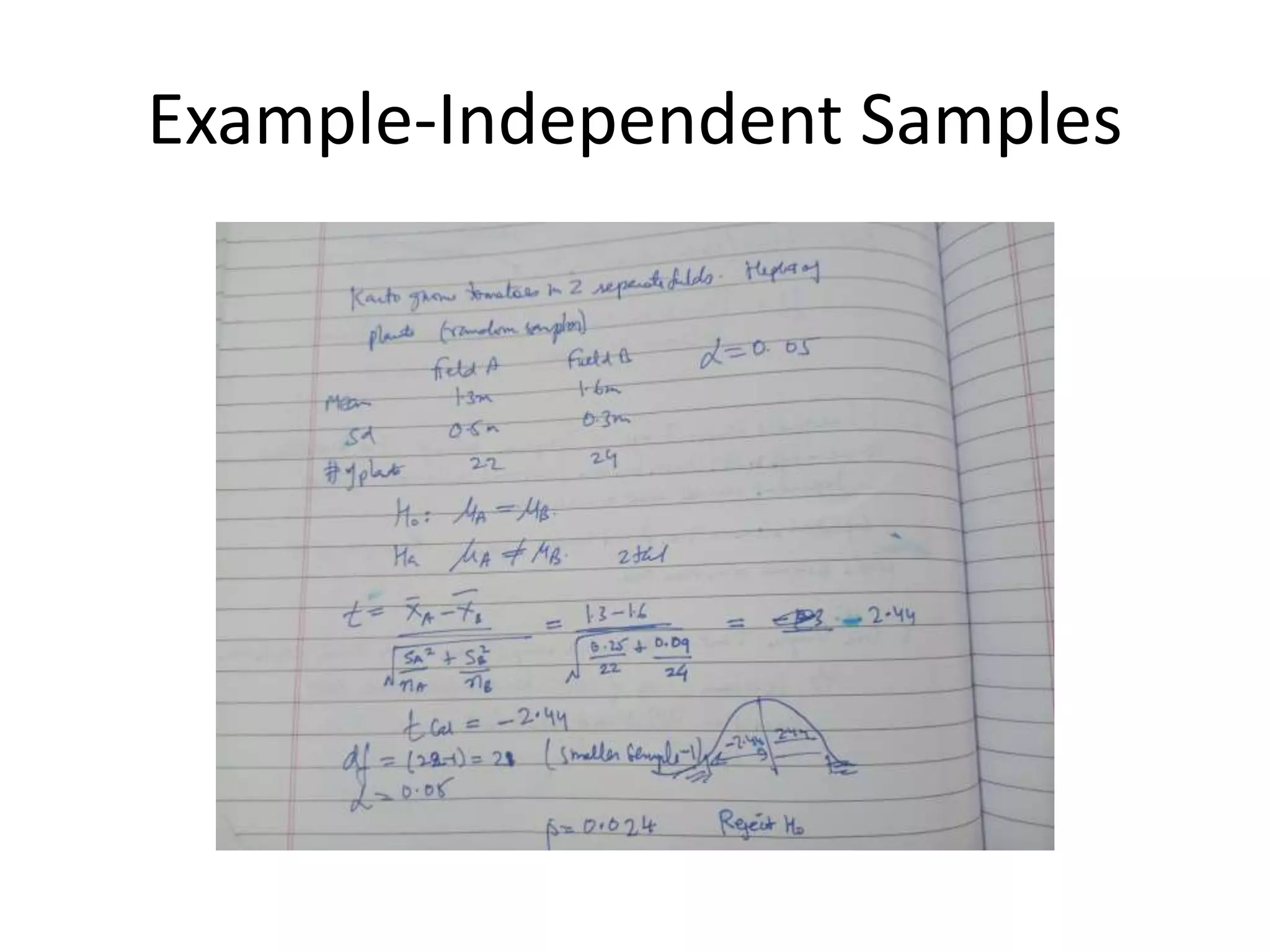
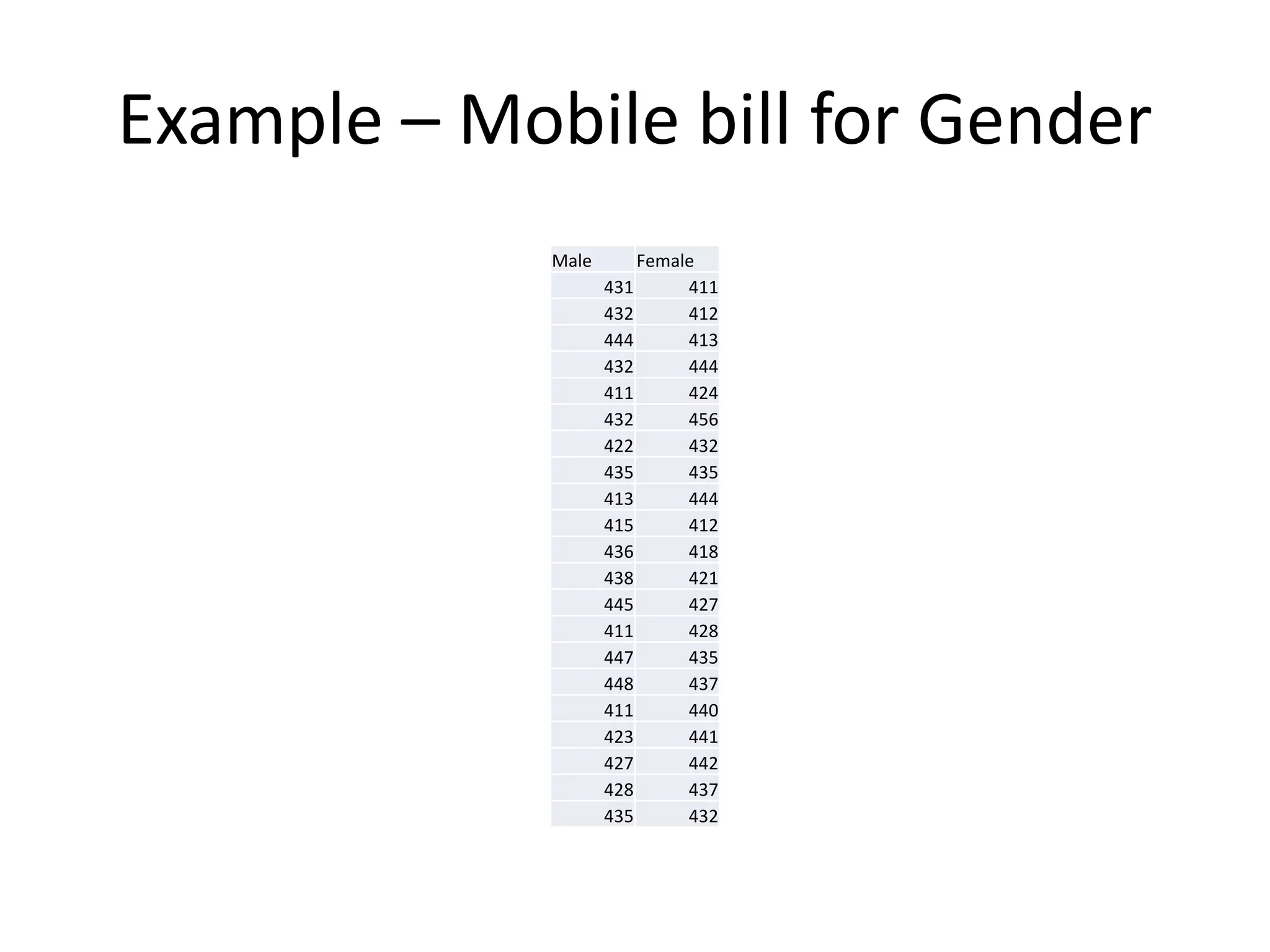
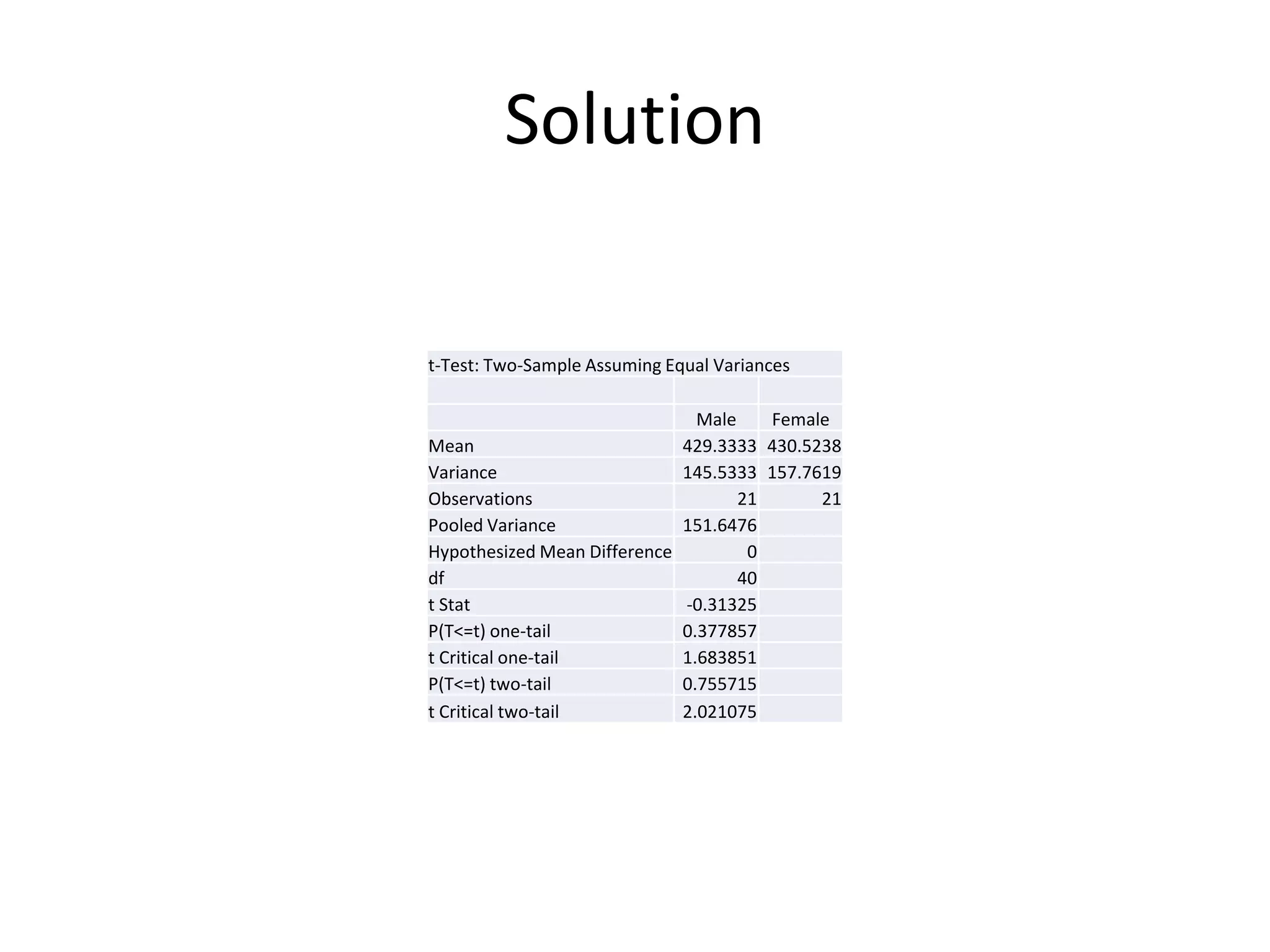
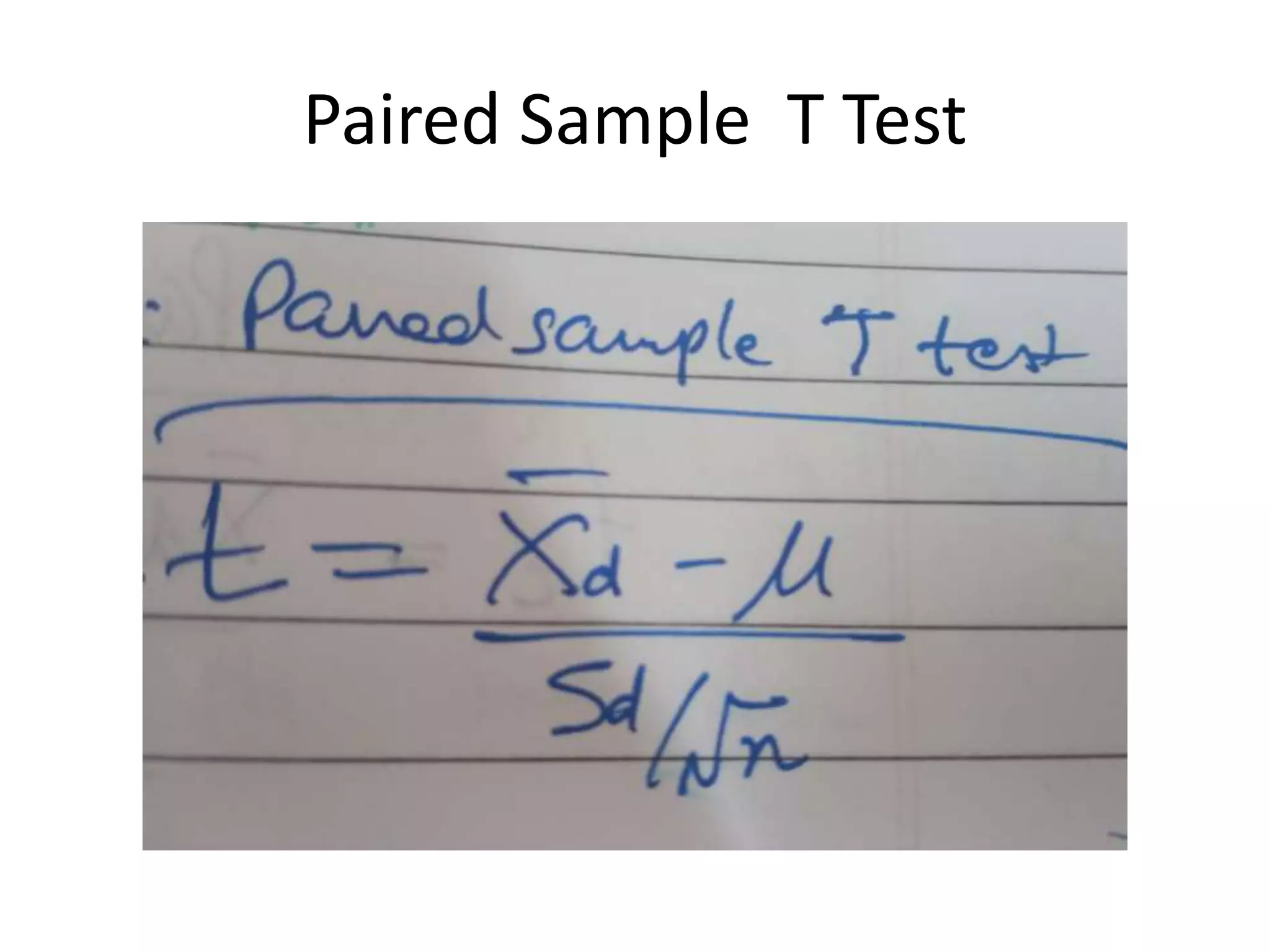
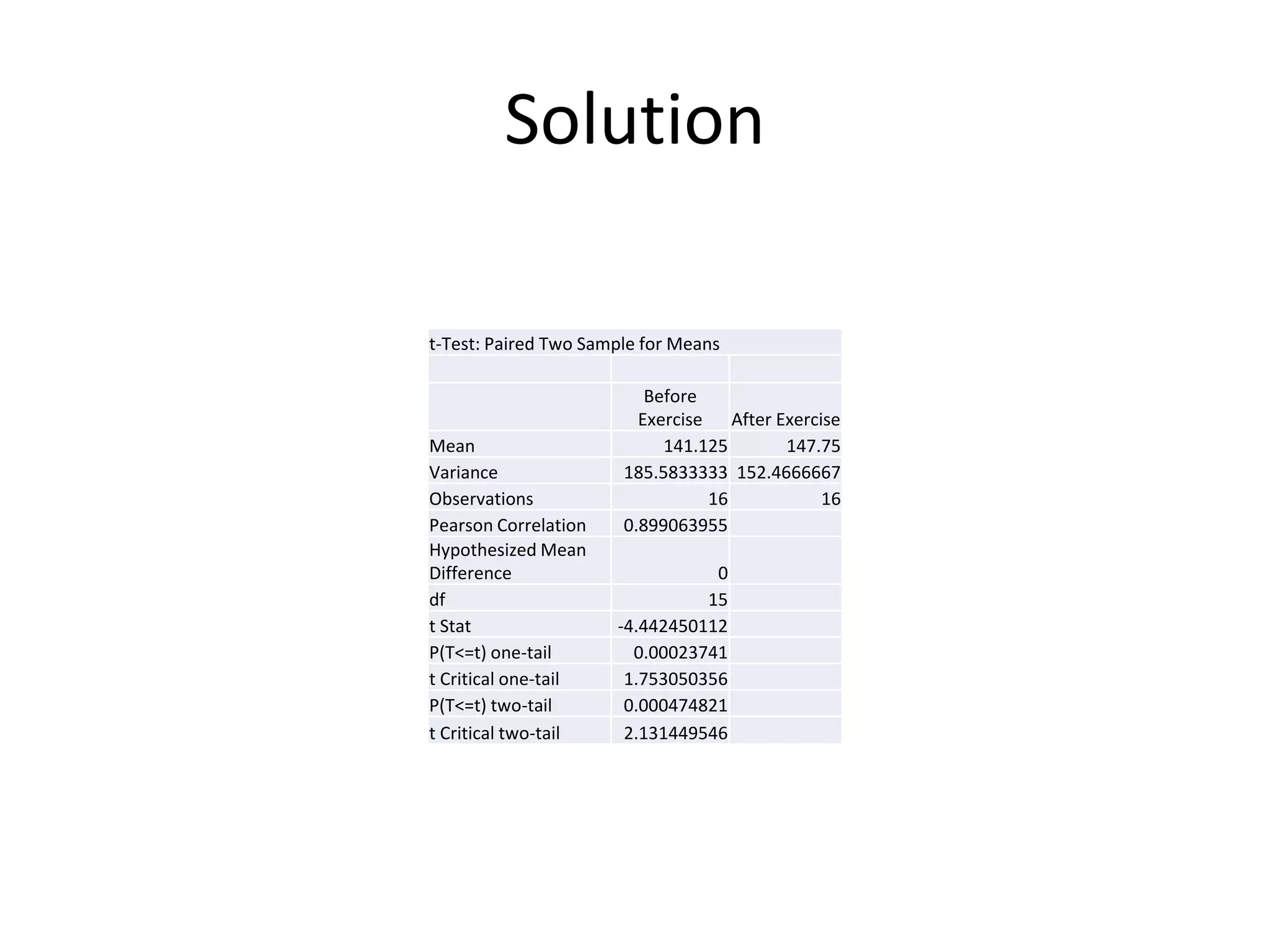
Hypothesis testing
t and Anova in Excel, SPSS and PSPP
What is the t-distribution?
Hypothesis Testing
• Likert Scale data
• Research Hypothesis & Statistical Hypothesis
• Check Normality of Data
• Choose Parametric /Non Parametric test
• Check p value for Ho or Ha depending on
confidence interval
Hypothesis Testing
 Null and Alternative Hypotheses
 Both Ho and Ha are statements about population
parameters, not sample statistics.
 A decision to retain the null hypothesis implies a lackof
support for the alternative hypothesis.
 A decision to reject the null hypothesis implies supportfor the
alternative hypothesis.
Hypothesis Testing
Sample Statistics - Hypothesized Parameter
Test Statistic =
Standard error of statistic
Types of Tests
Parametric Test
The statistical test which makes assumptions
about the distribution of population
parameters are known as parametric tests.
Non Parametric Test
The alternative which makes no assumptions
about the distribution of population
parameters are known as non parametric
tests.
Statistical
Techniques
Parametric
Statistics
Non Parametric
Statistics
Comparative Relationship
2 Groups > 2 Groups Covariate 2 Variables > 2 Variables Regression
ITT
DTT
OSTT
One Way
ANOVA
RM- ANOVA
Bet-Bet
ANOVA
Bet-With
ANOVA
With -With
ANOVA
ANOVA
Simple
Correlation
Multiple
Correlation
Partial
Correlation
Linear
Multiple
Logistic
2 Groups > 2 Groups
Mann
Whitney U
test
Wilcoxon
Rank Test
1 Sample
Sign Test
Kruskal-
Wallis H test
Friedman
Test
Rank Order
Correlation
Contingency
Coefficient
Phi
Correlation
Tetrachoric
Correlation
Point Biserial
Correlation
Biserial
Correlation
Goodness of
fit
Test for
independence
Statistical
Techniques
Parametric
Statistics
Non Parametric
Statistics
Comparative Relationship Others
Chi Square
P value
• The level in which we are allowed to
reject the null hypothesis when it is
true or Type 1 Error
• A rule of thumb is if p-value < 0.05
(5% level of significance) we reject
null hypothesis
• if p-value > 0.05 (5% level of
significance) we fail to reject null
hypothesis.
Tcal and Ttab to decide Hypothesis
• Tcal < Ttab – Fail to Reject Null Hypothesis
• Tcal>Ttab – Reject Null Hypothesis
Tcal , Zcal ,Fcal will be obtained from formulae
Ttab ,Ztab,Ftab will be obtained from Tables
All Software give Tcal,Fcal along with p values
Parametric Test
T Test
Z Test
F Test
Various types of T Test
One sample T Test
Independent sample T Test
Dependent sample T Test
T Test
In t-test, independent variable is
in nominal scale and
dependent variable
is in ratio scale.
One Sample T Test
• Null hypothesis: There is no significance
differences between the population mean and
the sample mean.
• In one sample T Test, a sample mean is compared
with the known population mean
Sample
Independent Sample T Test
• In Independent sample T Test, means of two
groups are compared.
• Null hypothesis: There is no significant difference
in means of two groups
Dependent Sample T Test
• In dependent sample T Test, means of same
group is compared before and after the
treatment.
• Null hypothesis: There is no significant difference
in means before and after treatment.
One Way ANOVA
• In Independent sample T Test, means of more
than three groups are compared.
• Null hypothesis: There is no significance
differences in marks of more than two groups
• One Sample T Tests
Hypothesis Testing Examples
Example : A normal white blood count is assumed to be approximately 8
thousand cells per cc of blood. A random sample of 15 employees of a nuclear
plant yielded a mean white count of 7.81 with a standard deviation of 0.872 (in
thousands).Is there significant evidence that the mean white count is lower for
plant employees using a=0.05?
Example : A pill is supposed to contain 20 mg of Phenobarbital. A random sample
of 29 pills yielded a mean of 20.5 mg and a standard deviation of 1.5 mg. Test
using a=0.10 whether the true mean amount per pill is 20 mg
Example: When a process producing ball bearings is operating correctly the
weights of the ball bearings have a normal distribution with mean 5 ounces and
standard deviation 0.1 ounce .An adjustment has been made to the process and
the plant manager suspects that this has raised the mean weight of ball bearings
produced leaving the standard deviation unchanged . A random sample of sixteen
ball bearings is taken, and their mean weight is found to be 5.038 ounces. Test at
significance levels .05 and .10 (that is, at 5% and 10% levels) that the adjustment
has not increased the mean weights of the ball bearings
6) When a process producing ball bearings is operating
correctly the weights of the ball bearings have a
normal distribution with mean 5 ounces and standard
deviation 0.1 ounce .An adjustment has been made to
the process and the plant manager suspects that this
has raised the mean weight of ball bearings produced
leaving the standard deviation unchanged . A random
sample of sixteen ball bearings is taken, and their
mean weight is found to be 5.038 ounces. Test at
significance levels .05 and .10 (that is, at 5% and 10%
levels) that the adjustment has not increased the mean
weights of the ball bearings
Independent Sample t test
Hypothesis –Independent Samples
Example-Independent Samples
Example – Mobile bill for Gender
Male Female
431 411
432 412
444 413
432 444
411 424
432 456
422 432
435 435
413 444
415 412
436 418
438 421
445 427
411 428
447 435
448 437
411 440
423 441
427 442
428 437
435 432
Solution
t-Test: Two-Sample Assuming Equal Variances
Male Female
Mean 429.3333 430.5238
Variance 145.5333 157.7619
Observations 21 21
Pooled Variance 151.6476
Hypothesized Mean Difference 0
df 40
t Stat -0.31325
P(T<=t) one-tail 0.377857
t Critical one-tail 1.683851
P(T<=t) two-tail 0.755715
t Critical two-tail 2.021075
Paired Sample T Test
Paired Sample T Test Example
Solution
Example
Proble
m Systolic Blood Pressure Before and After Exercise
Null Hypothesis : There is no difference in Systolic Blood Pressure Before and After Exercise
Alternative Hypothesis : There is a significance difference in Systolic Blood Pressure Before and After Exercise
Statistical Test : Dependent Sample t test /Paired 2 Sample for Means (Excel)
Before Exercise After Exercise
116 126
126 132
128 146
132 144
134 148
136 134
138 144
138 146
140 136
142 152
144 150
148 152
150 162
154 156
162 162
170 174
Solution
t-Test: Paired Two Sample for Means
Before
Exercise After Exercise
Mean 141.125 147.75
Variance 185.5833333 152.4666667
Observations 16 16
Pearson Correlation 0.899063955
Hypothesized Mean
Difference 0
df 15
t Stat -4.442450112
P(T<=t) one-tail 0.00023741
t Critical one-tail 1.753050356
P(T<=t) two-tail 0.000474821
t Critical two-tail 2.131449546

Topic 9 T Distribution.pptx

  • 1.
    Hypothesis testing t andAnova in Excel, SPSS and PSPP
  • 2.
    What is thet-distribution?
  • 10.
    Hypothesis Testing • LikertScale data • Research Hypothesis & Statistical Hypothesis • Check Normality of Data • Choose Parametric /Non Parametric test • Check p value for Ho or Ha depending on confidence interval
  • 11.
    Hypothesis Testing  Nulland Alternative Hypotheses  Both Ho and Ha are statements about population parameters, not sample statistics.  A decision to retain the null hypothesis implies a lackof support for the alternative hypothesis.  A decision to reject the null hypothesis implies supportfor the alternative hypothesis.
  • 12.
    Hypothesis Testing Sample Statistics- Hypothesized Parameter Test Statistic = Standard error of statistic
  • 13.
    Types of Tests ParametricTest The statistical test which makes assumptions about the distribution of population parameters are known as parametric tests. Non Parametric Test The alternative which makes no assumptions about the distribution of population parameters are known as non parametric tests.
  • 14.
    Statistical Techniques Parametric Statistics Non Parametric Statistics Comparative Relationship 2Groups > 2 Groups Covariate 2 Variables > 2 Variables Regression ITT DTT OSTT One Way ANOVA RM- ANOVA Bet-Bet ANOVA Bet-With ANOVA With -With ANOVA ANOVA Simple Correlation Multiple Correlation Partial Correlation Linear Multiple Logistic
  • 15.
    2 Groups >2 Groups Mann Whitney U test Wilcoxon Rank Test 1 Sample Sign Test Kruskal- Wallis H test Friedman Test Rank Order Correlation Contingency Coefficient Phi Correlation Tetrachoric Correlation Point Biserial Correlation Biserial Correlation Goodness of fit Test for independence Statistical Techniques Parametric Statistics Non Parametric Statistics Comparative Relationship Others Chi Square
  • 16.
    P value • Thelevel in which we are allowed to reject the null hypothesis when it is true or Type 1 Error • A rule of thumb is if p-value < 0.05 (5% level of significance) we reject null hypothesis • if p-value > 0.05 (5% level of significance) we fail to reject null hypothesis.
  • 18.
    Tcal and Ttabto decide Hypothesis • Tcal < Ttab – Fail to Reject Null Hypothesis • Tcal>Ttab – Reject Null Hypothesis Tcal , Zcal ,Fcal will be obtained from formulae Ttab ,Ztab,Ftab will be obtained from Tables All Software give Tcal,Fcal along with p values
  • 19.
  • 20.
    Various types ofT Test One sample T Test Independent sample T Test Dependent sample T Test
  • 21.
    T Test In t-test,independent variable is in nominal scale and dependent variable is in ratio scale.
  • 22.
    One Sample TTest • Null hypothesis: There is no significance differences between the population mean and the sample mean. • In one sample T Test, a sample mean is compared with the known population mean Sample
  • 23.
    Independent Sample TTest • In Independent sample T Test, means of two groups are compared. • Null hypothesis: There is no significant difference in means of two groups
  • 24.
    Dependent Sample TTest • In dependent sample T Test, means of same group is compared before and after the treatment. • Null hypothesis: There is no significant difference in means before and after treatment.
  • 25.
    One Way ANOVA •In Independent sample T Test, means of more than three groups are compared. • Null hypothesis: There is no significance differences in marks of more than two groups
  • 26.
  • 32.
    Hypothesis Testing Examples Example: A normal white blood count is assumed to be approximately 8 thousand cells per cc of blood. A random sample of 15 employees of a nuclear plant yielded a mean white count of 7.81 with a standard deviation of 0.872 (in thousands).Is there significant evidence that the mean white count is lower for plant employees using a=0.05? Example : A pill is supposed to contain 20 mg of Phenobarbital. A random sample of 29 pills yielded a mean of 20.5 mg and a standard deviation of 1.5 mg. Test using a=0.10 whether the true mean amount per pill is 20 mg Example: When a process producing ball bearings is operating correctly the weights of the ball bearings have a normal distribution with mean 5 ounces and standard deviation 0.1 ounce .An adjustment has been made to the process and the plant manager suspects that this has raised the mean weight of ball bearings produced leaving the standard deviation unchanged . A random sample of sixteen ball bearings is taken, and their mean weight is found to be 5.038 ounces. Test at significance levels .05 and .10 (that is, at 5% and 10% levels) that the adjustment has not increased the mean weights of the ball bearings
  • 33.
    6) When aprocess producing ball bearings is operating correctly the weights of the ball bearings have a normal distribution with mean 5 ounces and standard deviation 0.1 ounce .An adjustment has been made to the process and the plant manager suspects that this has raised the mean weight of ball bearings produced leaving the standard deviation unchanged . A random sample of sixteen ball bearings is taken, and their mean weight is found to be 5.038 ounces. Test at significance levels .05 and .10 (that is, at 5% and 10% levels) that the adjustment has not increased the mean weights of the ball bearings
  • 34.
  • 36.
  • 37.
  • 38.
    Example – Mobilebill for Gender Male Female 431 411 432 412 444 413 432 444 411 424 432 456 422 432 435 435 413 444 415 412 436 418 438 421 445 427 411 428 447 435 448 437 411 440 423 441 427 442 428 437 435 432
  • 39.
    Solution t-Test: Two-Sample AssumingEqual Variances Male Female Mean 429.3333 430.5238 Variance 145.5333 157.7619 Observations 21 21 Pooled Variance 151.6476 Hypothesized Mean Difference 0 df 40 t Stat -0.31325 P(T<=t) one-tail 0.377857 t Critical one-tail 1.683851 P(T<=t) two-tail 0.755715 t Critical two-tail 2.021075
  • 40.
  • 41.
  • 42.
    Paired Sample TTest Example
  • 43.
  • 44.
    Example Proble m Systolic BloodPressure Before and After Exercise Null Hypothesis : There is no difference in Systolic Blood Pressure Before and After Exercise Alternative Hypothesis : There is a significance difference in Systolic Blood Pressure Before and After Exercise Statistical Test : Dependent Sample t test /Paired 2 Sample for Means (Excel) Before Exercise After Exercise 116 126 126 132 128 146 132 144 134 148 136 134 138 144 138 146 140 136 142 152 144 150 148 152 150 162 154 156 162 162 170 174
  • 45.
    Solution t-Test: Paired TwoSample for Means Before Exercise After Exercise Mean 141.125 147.75 Variance 185.5833333 152.4666667 Observations 16 16 Pearson Correlation 0.899063955 Hypothesized Mean Difference 0 df 15 t Stat -4.442450112 P(T<=t) one-tail 0.00023741 t Critical one-tail 1.753050356 P(T<=t) two-tail 0.000474821 t Critical two-tail 2.131449546