Concepts & Definition
•It is the inductive process of inferring the
population characteristics based on the sample
outcomes using different statistical techniques.
• It helps the determination of
difference/similarities found between group or
groups and it is expressed in terms of statistical
significance.
• Few concepts related to the inferential statistics
are;
3.
Classification
• Inferential statisticsis broadly classified into;
• A. Estimation
• B. Test of significance.
A. Estimation.
• It is the process of quantifying a study characteristics either as a
point estimation or interval estimation.
• Point estimation use a particular point/single value (Eg. 50%
people are rich), whereas interval estimation uses two limits with
the attached probability (Eg. The heart rate of normal individual
is 60 to 80 (with 95% of probability))
4.
Classification
B. Test ofSignificance.
• It is the process of quantifying a study
characteristics with the help of statistical
techniques. (Hypothesis testing).
5.
Hypothesis: Types
Based onStatistical Purpose
• Null Hypothesis: A hypothesis stating no difference
or no relation between the variables is known as
null hypothesis. (H0)
• Alternative Hypothesis: A hypothesis stating
presence of difference or relation between the
variables is known as alternative hypothesis. (H1 ,
H2)
6.
Hypothesis: Types
Based onNumber of Variables
• Simple Hypothesis: A hypothesis stating one to one
correspondence relationship between two variables is called
as simple variable. (Eg. There is significant correlation
between gestational age and systolic BP.)
• Composite Hypothesis: It is the statement of relationship
between one to many or many to one variable. (Eg. Birth
weight may be related to maternal age, gestational age,
gestational weight gain, tobacco smoking, alcoholism etc.)
7.
Type I andType II Errors
• Type I Error: It occurs when null hypothesis is rejected,
where it should have been accepted. The probability of
making a type I error is α (alpha error), which is the level of
significance you set for your hypothesis test. An α (alpha) of
0.05 indicates that you are willing to accept a 5% chance
that you are wrong when you reject the null hypothesis.
• Type II Error: It occurs when the null hypothesis is false
and you fail to reject it. The probability of making a type II
error is β, which depends on the power of the test. This can
be avoided by increasing the sample size and using the
proper statistical techniques.
8.
Level of Significance
•Probability of making Type I error is called as level of
significance.
• It is denoted by “α” (alpha) or “p”.
• It is the probability of rejecting the null hypothesis when it is
true.
• In health sciences we generally consider either 1% (0.01) or
5% (0.05) as significance.
• It shows the risk of being wrong in decision is explained in
terms of 1 in 100 or 5 in 100.
• 1 is understood as more effective and accurate when the
significance is 0.01 compare to 0.05.
9.
Confidence Interval
• Aconfidence interval is a range of values, with a specified
degree of probability is thought to contain the population
value.
• It is a method of assertion that a particular population
parameter lies within those specified boundaries.
• It is required to be calculated since the analysis is done on
sample not on population.
• The CI contains a lower and upper limit between which the
parameter is expected to fall.
10.
Confidence Interval
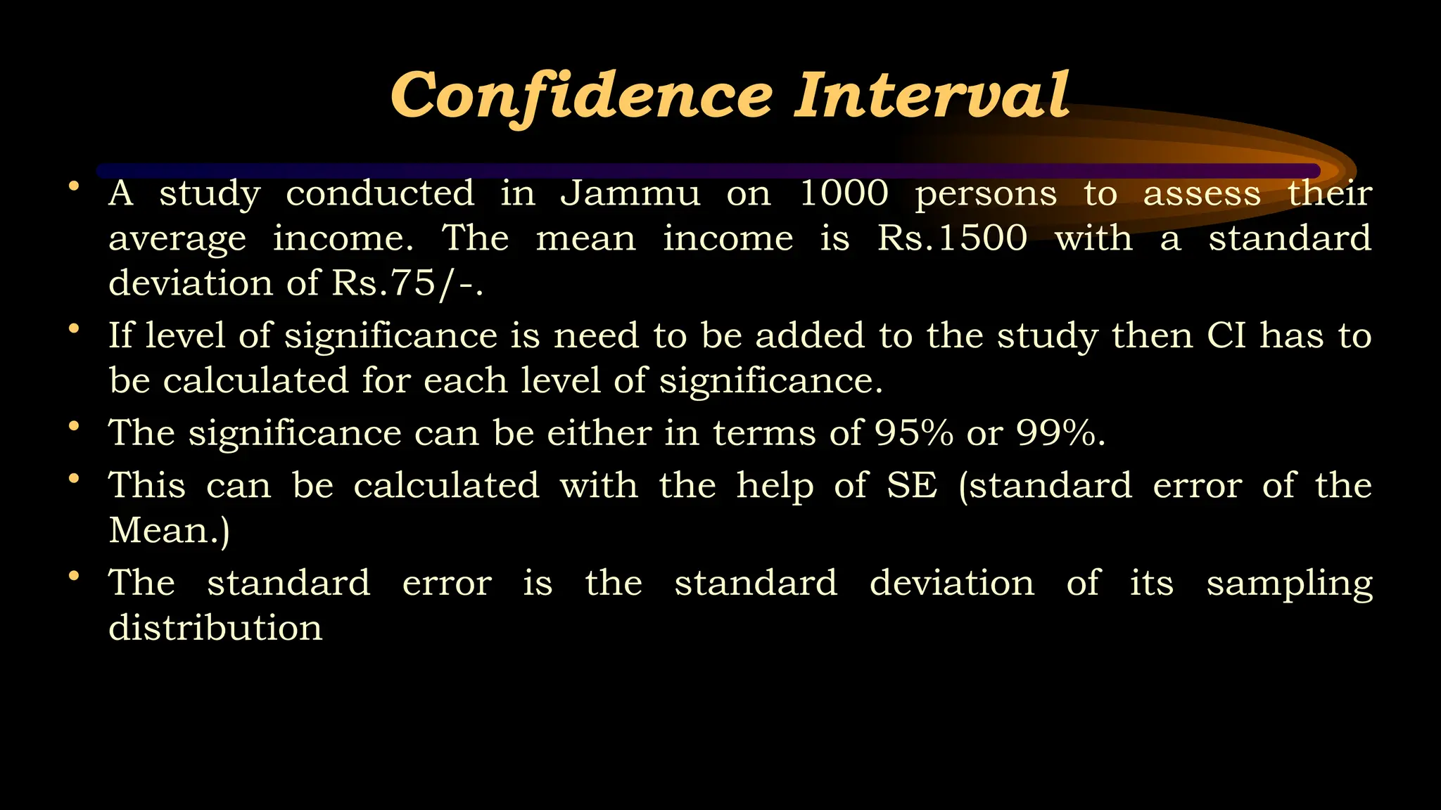
• Astudy conducted in Jammu on 1000 persons to assess their
average income. The mean income is Rs.1500 with a standard
deviation of Rs.75/-.
• If level of significance is need to be added to the study then CI has to
be calculated for each level of significance.
• The significance can be either in terms of 95% or 99%.
• This can be calculated with the help of SE (standard error of the
Mean.)
• The standard error is the standard deviation of its sampling
distribution
11.
Confidence Interval
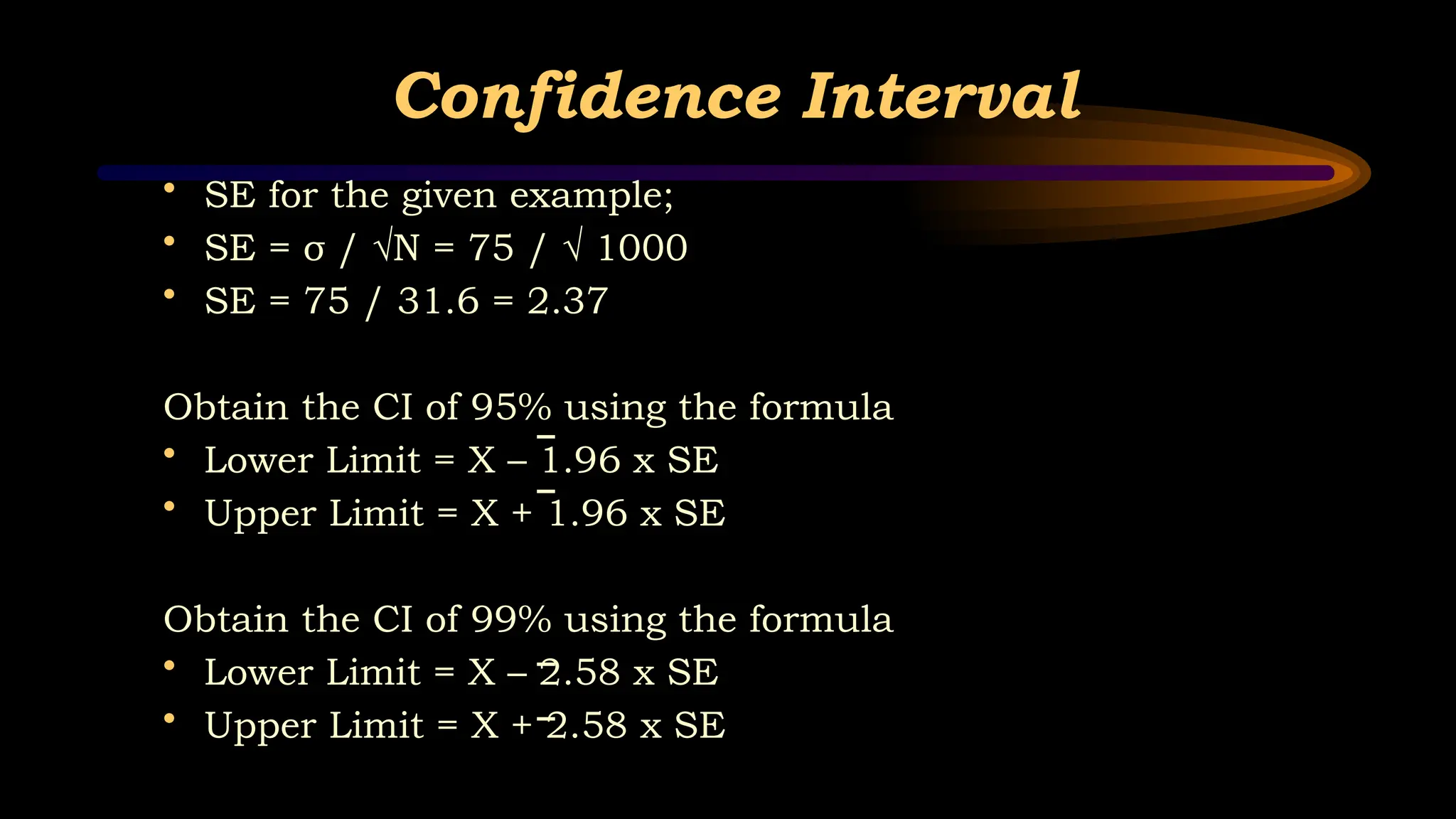
• SEfor the given example;
• SE = σ / √N = 75 / √ 1000
• SE = 75 / 31.6 = 2.37
Obtain the CI of 95% using the formula
• Lower Limit = X – 1.96 x SE
• Upper Limit = X + 1.96 x SE
Obtain the CI of 99% using the formula
• Lower Limit = X – 2.58 x SE
• Upper Limit = X + 2.58 x SE
12.
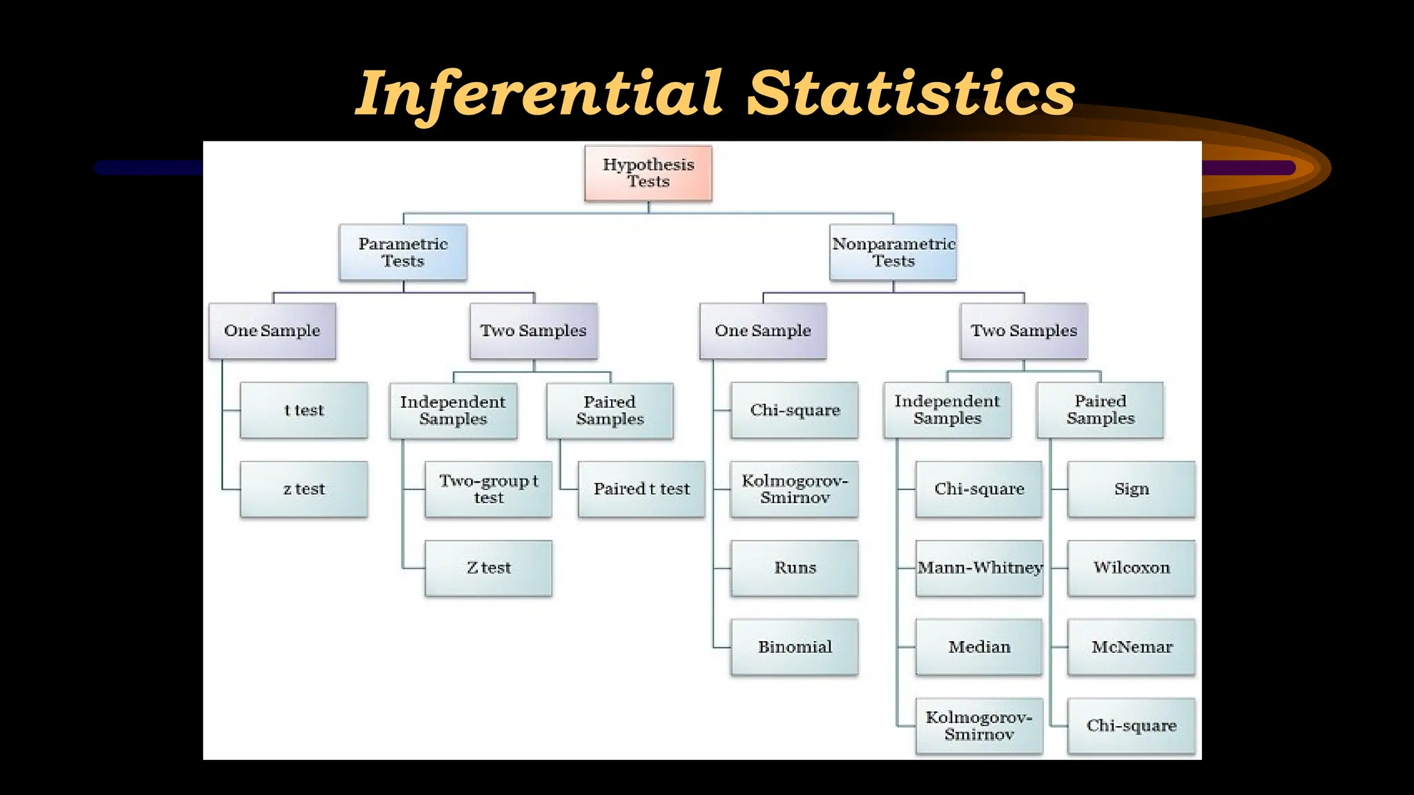
Inferential Statistics
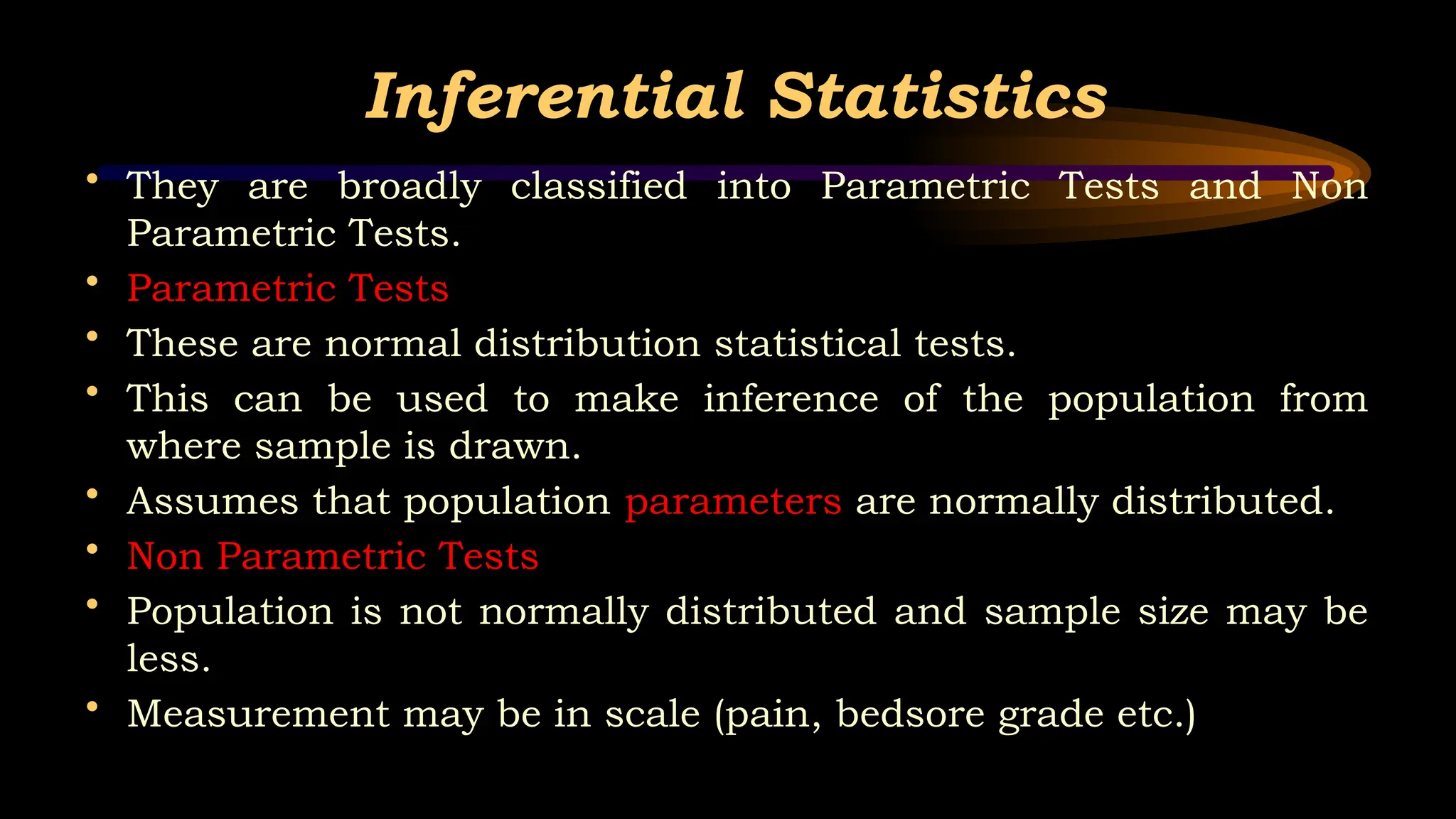
• Theyare broadly classified into Parametric Tests and Non
Parametric Tests.
• Parametric Tests
• These are normal distribution statistical tests.
• This can be used to make inference of the population from
where sample is drawn.
• Assumes that population parameters are normally distributed.
• Non Parametric Tests
• Population is not normally distributed and sample size may be
less.
• Measurement may be in scale (pain, bedsore grade etc.)
13.
Comparison Chart
BASIS FOR
COMPARISON
PARAMETRICTEST
NONPARAMETRIC
TEST
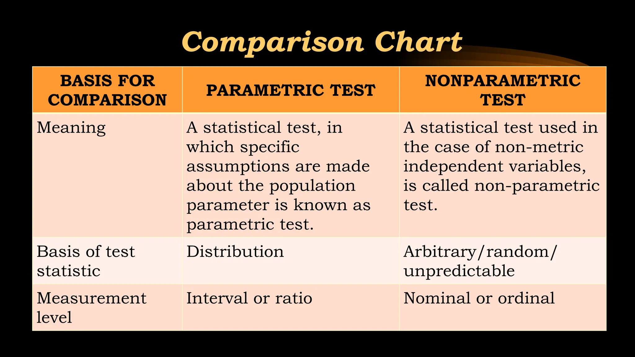
Meaning A statistical test, in
which specific
assumptions are made
about the population
parameter is known as
parametric test.
A statistical test used in
the case of non-metric
independent variables,
is called non-parametric
test.
Basis of test
statistic
Distribution Arbitrary/random/
unpredictable
Measurement
level
Interval or ratio Nominal or ordinal
14.
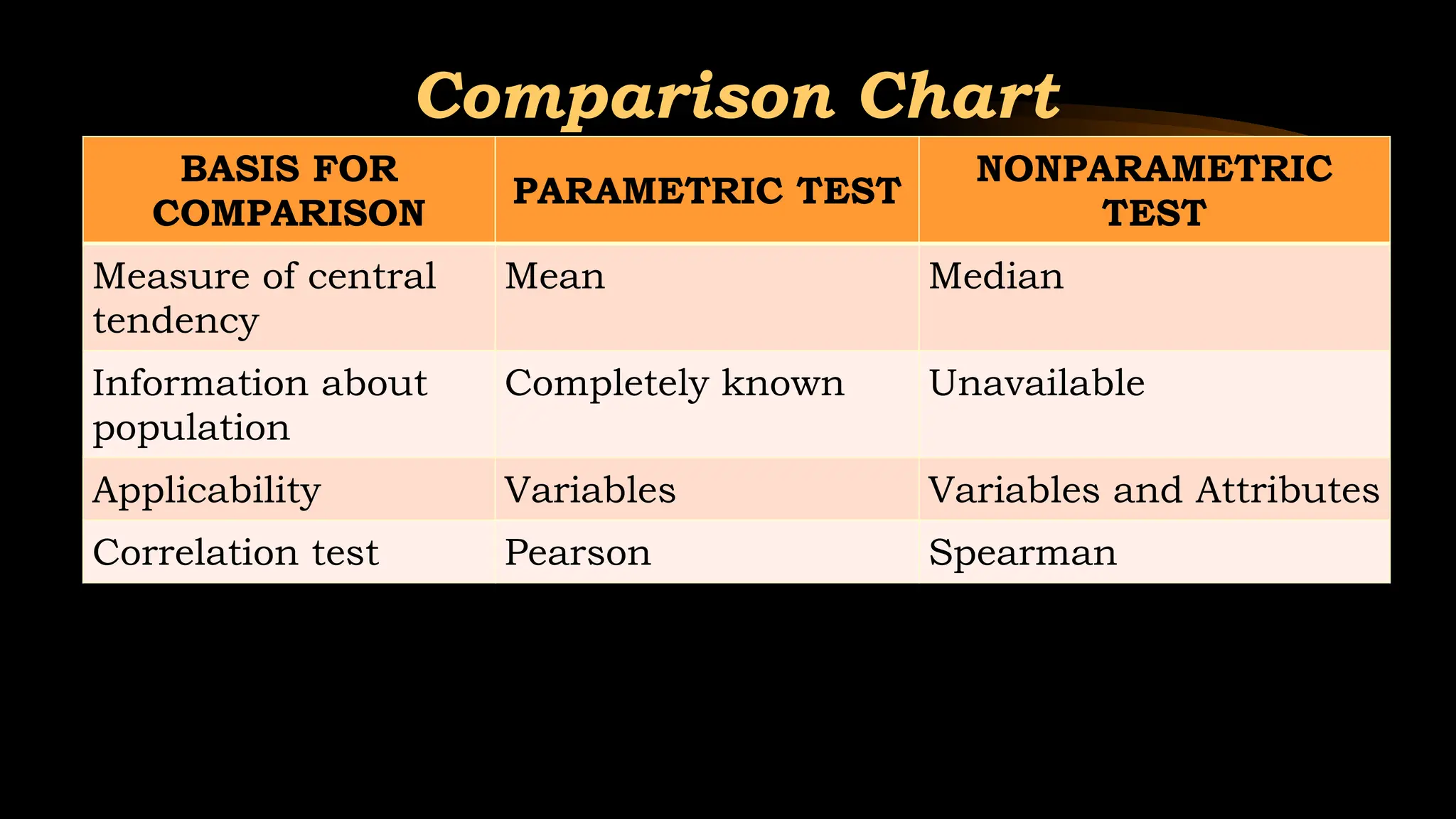
Comparison Chart
BASIS FOR
COMPARISON
PARAMETRICTEST
NONPARAMETRIC
TEST
Measure of central
tendency
Mean Median
Information about
population
Completely known Unavailable
Applicability Variables Variables and Attributes
Correlation test Pearson Spearman
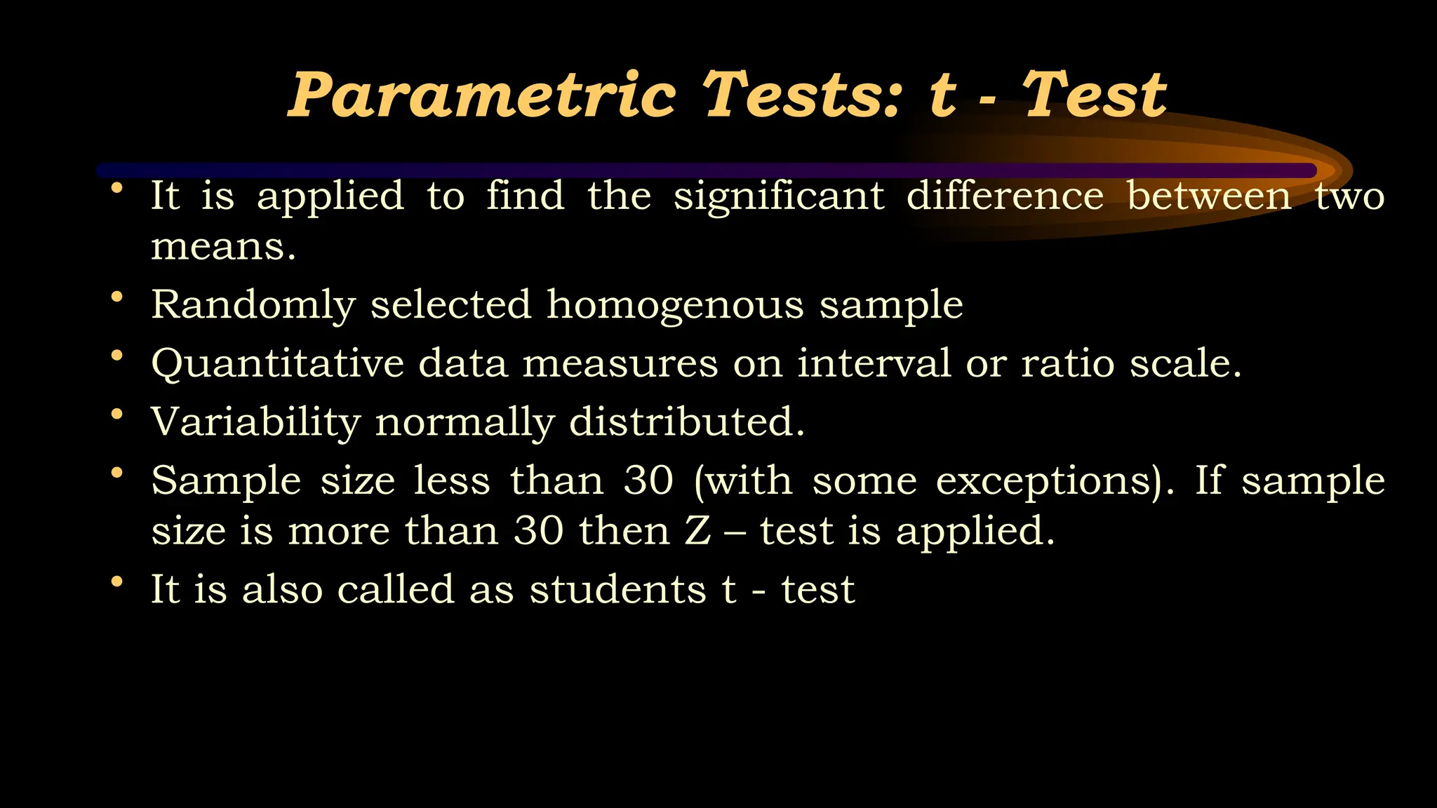
Parametric Tests: t- Test
• It is applied to find the significant difference between two
means.
• Randomly selected homogenous sample
• Quantitative data measures on interval or ratio scale.
• Variability normally distributed.
• Sample size less than 30 (with some exceptions). If sample
size is more than 30 then Z – test is applied.
• It is also called as students t - test
18.
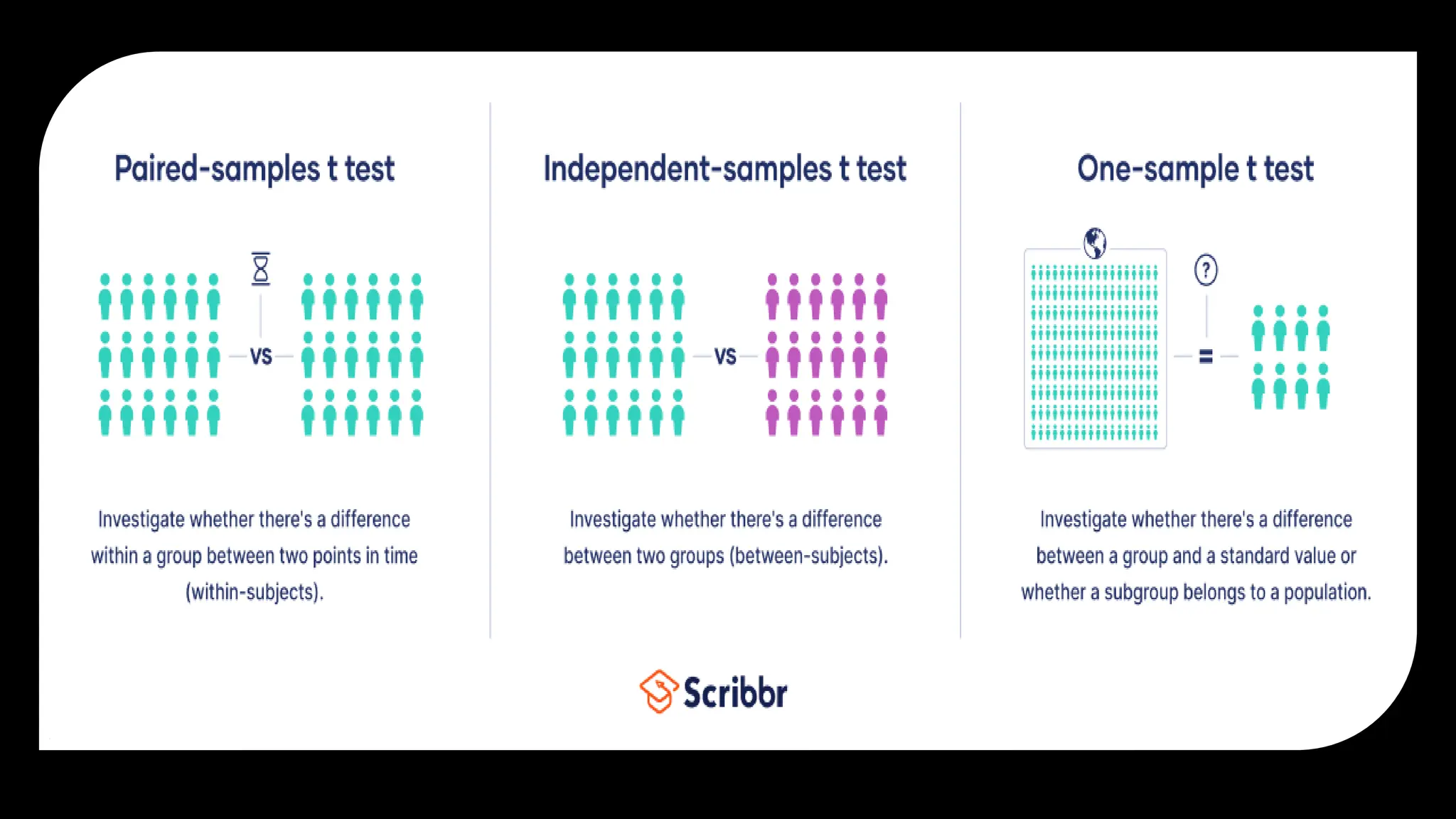
Parametric Tests: t- Test
• Types of t – Tests.
• 1. Unpaired t-Test: It is applied when we obtain data from
subjects of two independent separated groups of people or
samples drawn from two types of population.
• 2. Paired t-Test: It is applied on paired data of
independent observations made on same sample before and
after the intervention. It is commonly used in nursing
studies.
19.
Unpaired t -Test
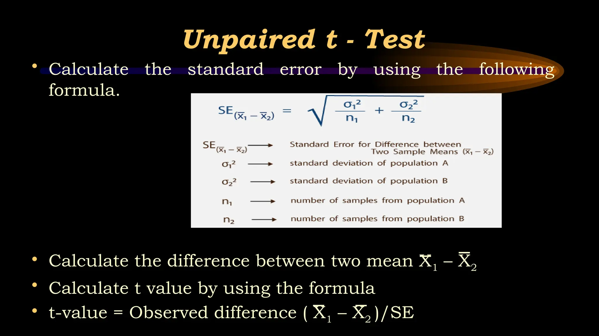
• Calculate the standard error by using the following
formula.
• Calculate the difference between two mean X1 – X2
• Calculate t value by using the formula
• t-value = Observed difference ( X1 – X2 )/SE
20.
Unpaired t -Test
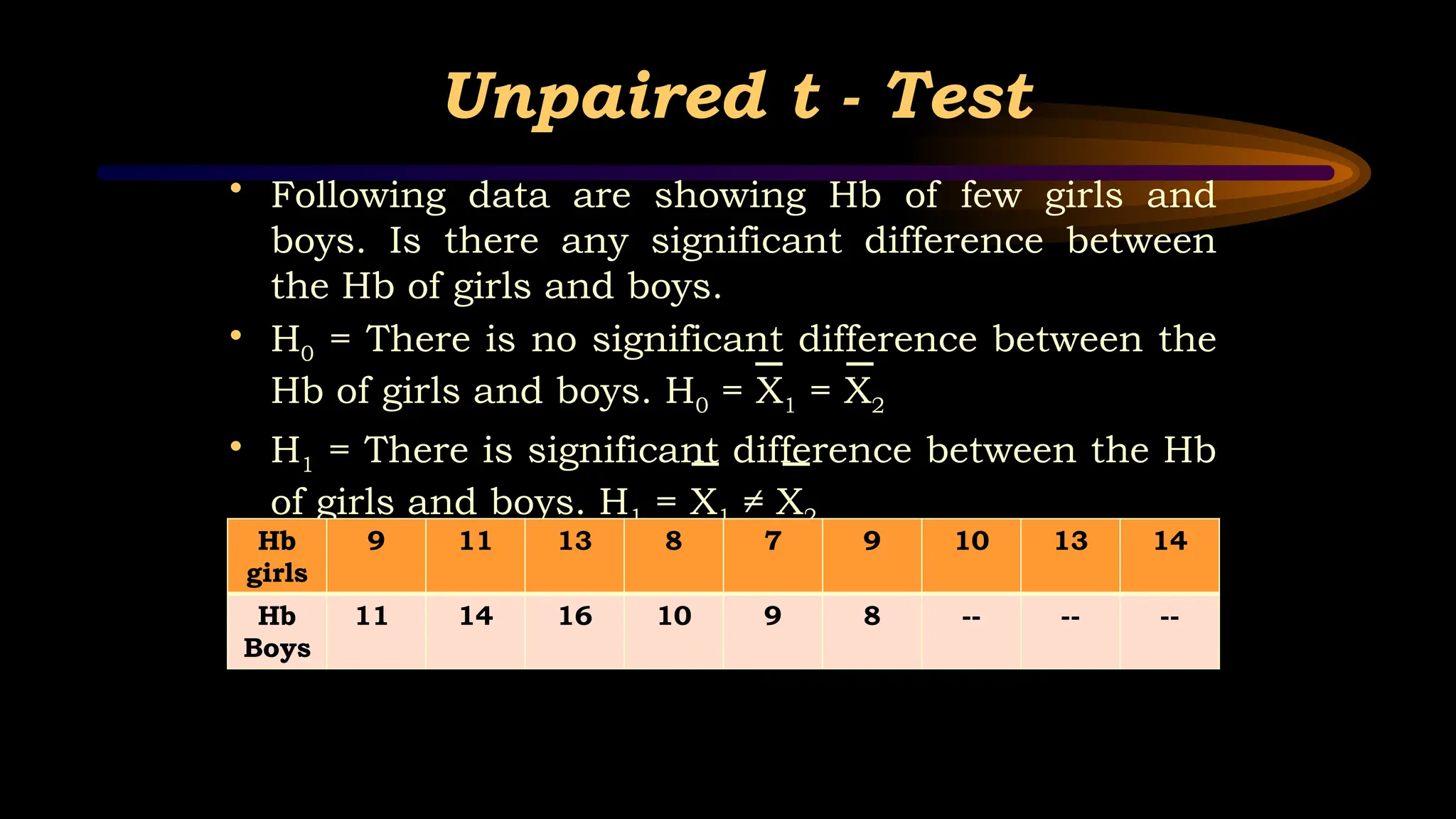
• Following data are showing Hb of few girls and
boys. Is there any significant difference between
the Hb of girls and boys.
• H0 = There is no significant difference between the
Hb of girls and boys. H0 = X1 = X2
• H1 = There is significant difference between the Hb
of girls and boys. H1 = X1 ≠ X2
Hb
girls
9 11 13 8 7 9 10 13 14
Hb
Boys
11 14 16 10 9 8 -- -- --
21.
Unpaired t -Test
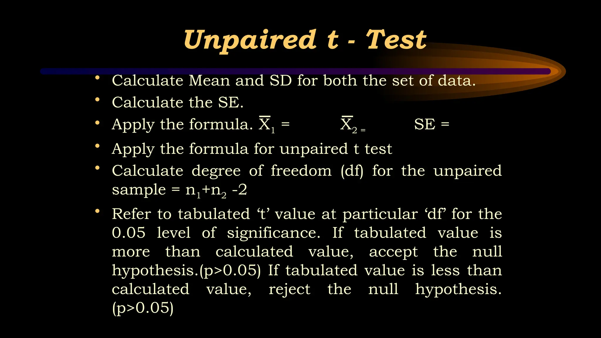
• Calculate Mean and SD for both the set of data.
• Calculate the SE.
• Apply the formula. X1 = X2 = SE =
• Apply the formula for unpaired t test
• Calculate degree of freedom (df) for the unpaired
sample = n1+n2 -2
• Refer to tabulated ‘t’ value at particular ‘df’ for the
0.05 level of significance. If tabulated value is
more than calculated value, accept the null
hypothesis.(p>0.05) If tabulated value is less than
calculated value, reject the null hypothesis.
(p>0.05)
22.
One tail VsTwo tail tests
• A two-tailed test is appropriate if the estimated value may
be more than or less than the reference value, for
example, whether a test taker may score above or below
the historical average. Eg. H1 = There is significant
difference between the Hb of girls and boys
• A one-tailed test is appropriate if the estimated value may
depart from the reference value in only one direction, for
example, such as increasing or decreasing but not on
both direction. Eg. H1 = There is significant increase in
the BP of patients after the particular intervention.
23.
Paired t -Test
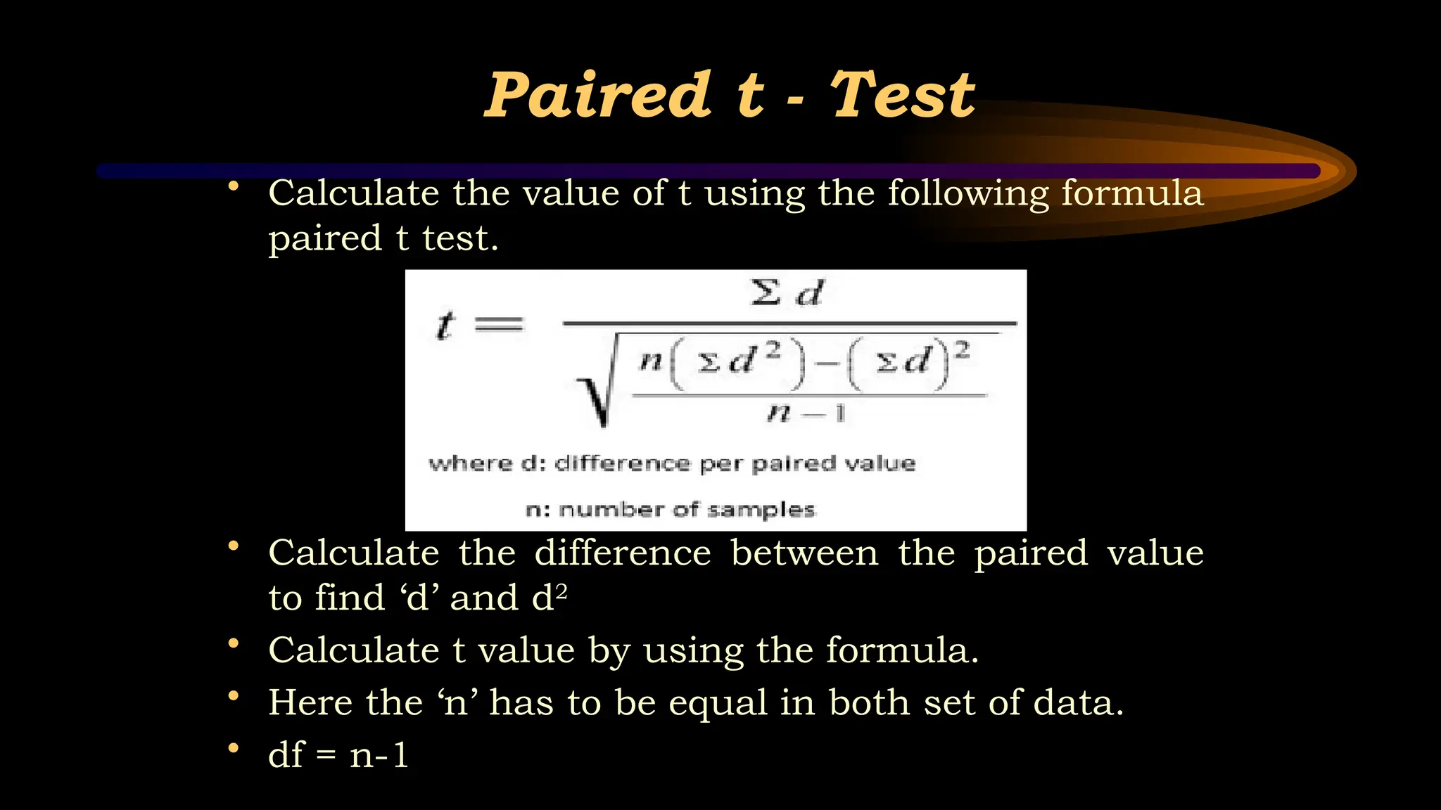
• Calculate the value of t using the following formula
paired t test.
• Calculate the difference between the paired value
to find ‘d’ and d2
• Calculate t value by using the formula.
• Here the ‘n’ has to be equal in both set of data.
• df = n-1
24.
Paired t -Test
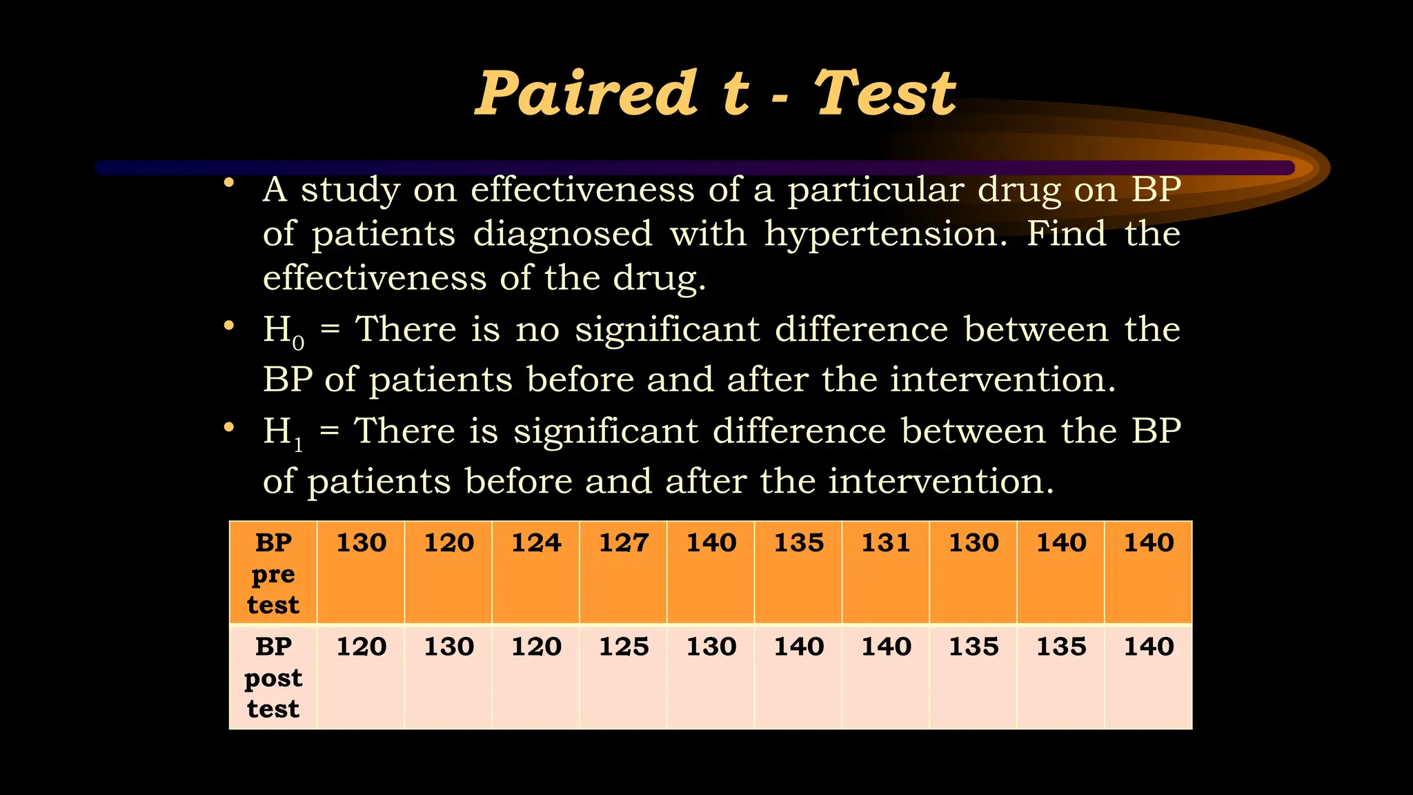
• A study on effectiveness of a particular drug on BP
of patients diagnosed with hypertension. Find the
effectiveness of the drug.
• H0 = There is no significant difference between the
BP of patients before and after the intervention.
• H1 = There is significant difference between the BP
of patients before and after the intervention.
BP
pre
test
130 120 124 127 140 135 131 130 140 140
BP
post
test
120 130 120 125 130 140 140 135 135 140
25.
Paired t -Test
• Calculate Mean and d and d2
for both the set of
data.
• Apply the formula.
• Apply the formula for unpaired t test
• Calculate degree of freedom (df) for the paired
sample = n -1
• Refer to tabulated ‘t’ value at particular ‘df’ for the
0.05 level of significance. If tabulated value is
more than calculated value, accept the null
hypothesis.(p>0.05) If tabulated value is less than
calculated value, reject the null hypothesis.
(p>0.05)
26.
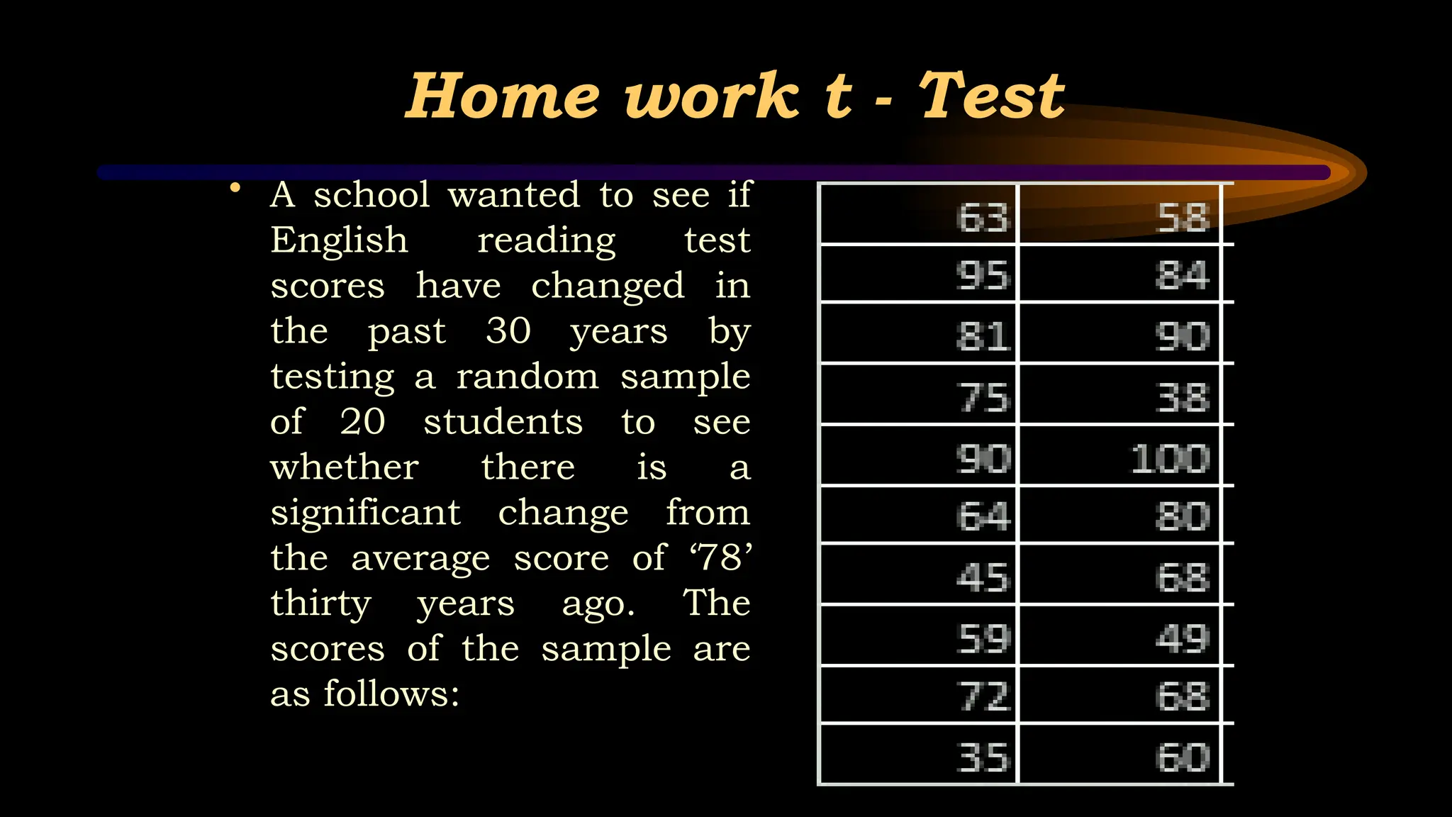
Home work t- Test
• A school wanted to see if
English reading test
scores have changed in
the past 30 years by
testing a random sample
of 20 students to see
whether there is a
significant change from
the average score of ‘78’
thirty years ago. The
scores of the sample are
as follows:
27.
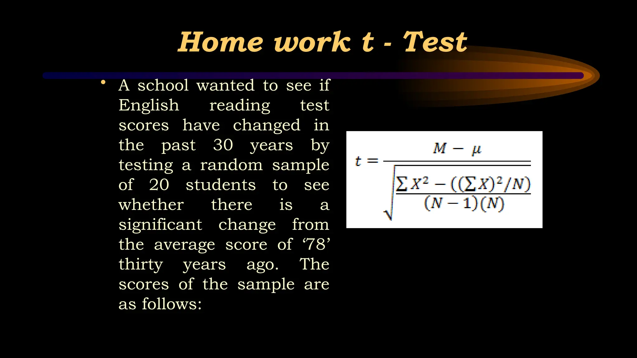
Home work t- Test
• A school wanted to see if
English reading test
scores have changed in
the past 30 years by
testing a random sample
of 20 students to see
whether there is a
significant change from
the average score of ‘78’
thirty years ago. The
scores of the sample are
as follows:
28.
Z - Test
•When the sample is larger than 30 subjects and
the researcher wants to compare the difference in
a population mean and a sample mean or two
sample means.
• The samples should be randomly collected.
• The data must be quantitative in terms of interval
or ratio.
• The variability is assumed to follow normal
distribution.
• Sample size more than 30.
29.
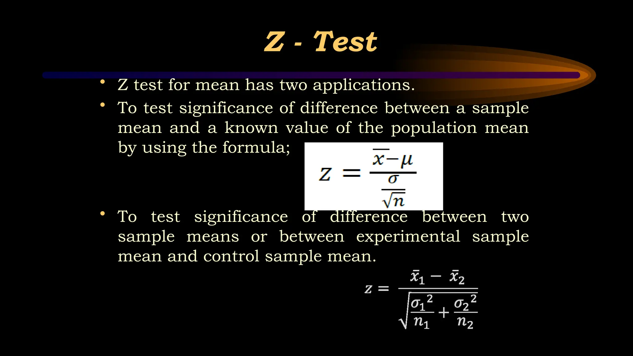
Z - Test
•Z test for mean has two applications.
• To test significance of difference between a sample
mean and a known value of the population mean
by using the formula;
• To test significance of difference between two
sample means or between experimental sample
mean and control sample mean.
30.
Z - Test
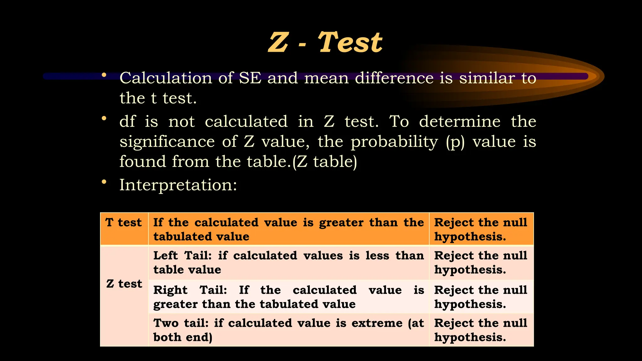
•Calculation of SE and mean difference is similar to
the t test.
• df is not calculated in Z test. To determine the
significance of Z value, the probability (p) value is
found from the table.(Z table)
• Interpretation:
T test If the calculated value is greater than the
tabulated value
Reject the null
hypothesis.
Z test
Left Tail: if calculated values is less than
table value
Reject the null
hypothesis.
Right Tail: If the calculated value is
greater than the tabulated value
Reject the null
hypothesis.
Two tail: if calculated value is extreme (at
both end)
Reject the null
hypothesis.
31.
Z - Test
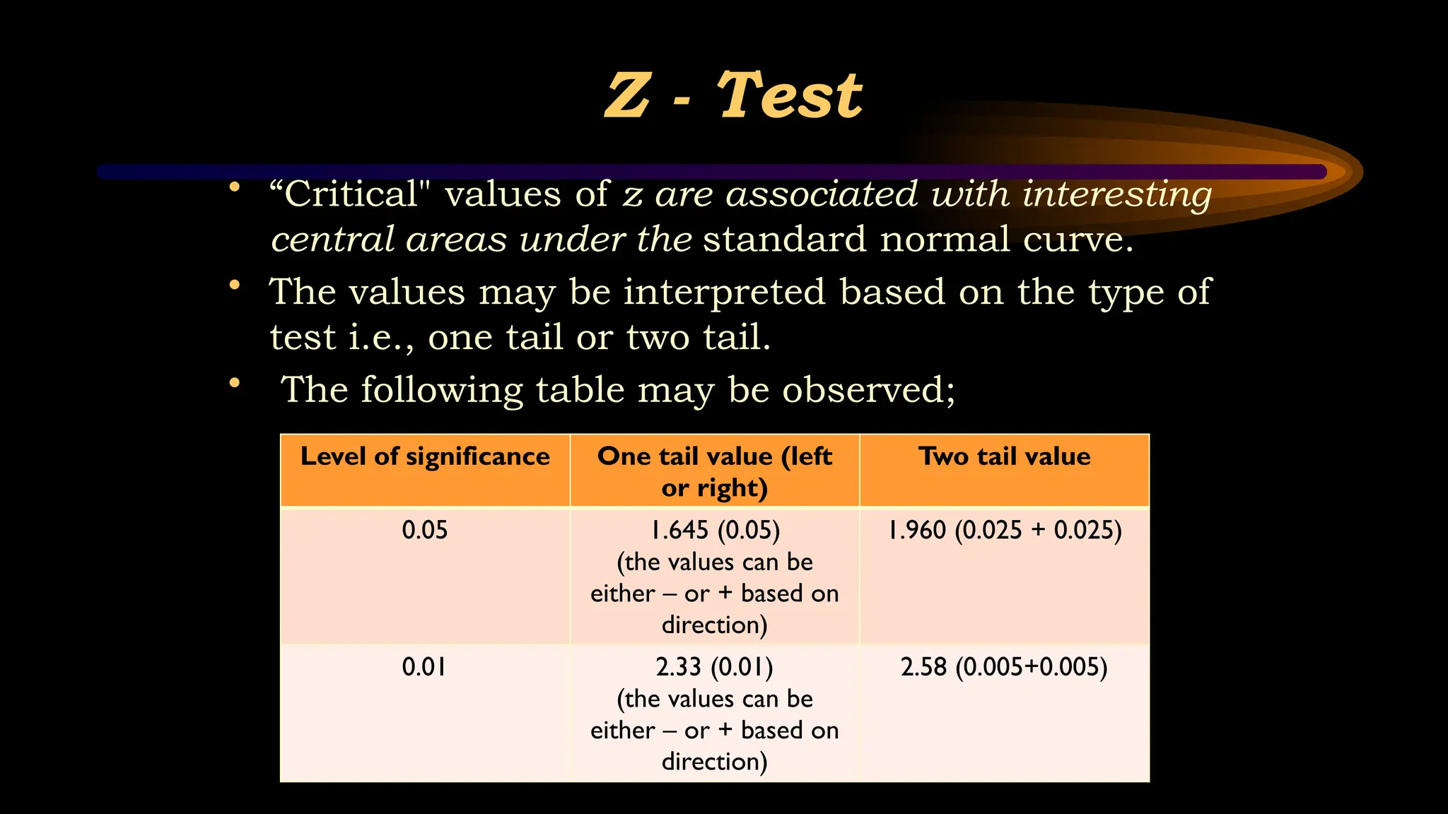
•“Critical" values of z are associated with interesting
central areas under the standard normal curve.
• The values may be interpreted based on the type of
test i.e., one tail or two tail.
• The following table may be observed;
Level of significance One tail value (left
or right)
Two tail value
0.05 1.645 (0.05)
(the values can be
either – or + based on
direction)
1.960 (0.025 + 0.025)
0.01 2.33 (0.01)
(the values can be
either – or + based on
direction)
2.58 (0.005+0.005)
32.
Z – Test:Example
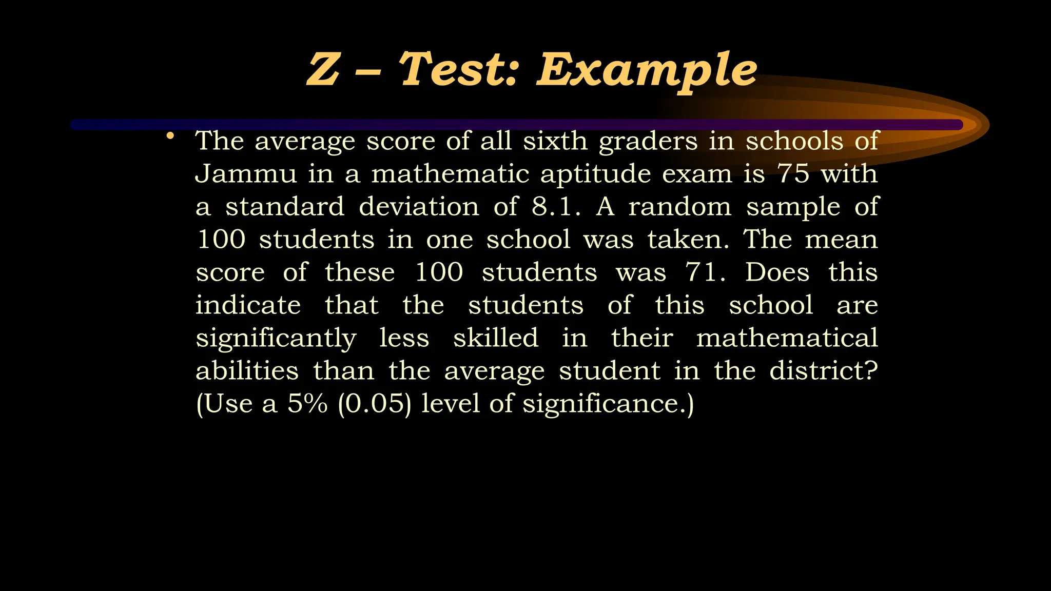
• The average score of all sixth graders in schools of
Jammu in a mathematic aptitude exam is 75 with
a standard deviation of 8.1. A random sample of
100 students in one school was taken. The mean
score of these 100 students was 71. Does this
indicate that the students of this school are
significantly less skilled in their mathematical
abilities than the average student in the district?
(Use a 5% (0.05) level of significance.)
33.
Z – Test:Example
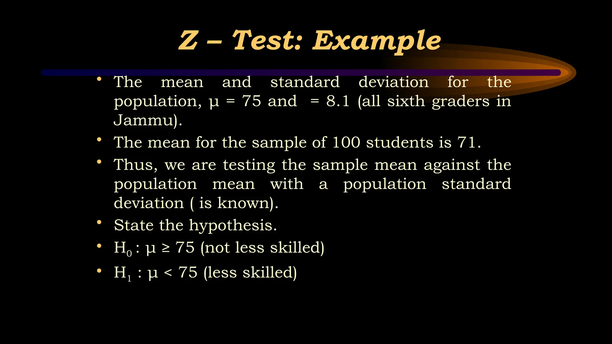
• The mean and standard deviation for the
population, μ = 75 and = 8.1 (all sixth graders in
Jammu).
• The mean for the sample of 100 students is 71.
• Thus, we are testing the sample mean against the
population mean with a population standard
deviation ( is known).
• State the hypothesis.
• H0 : μ ≥ 75 (not less skilled)
• H1 : μ < 75 (less skilled)
34.
Z – Test:Example
• Formulate decision rule: Since the alternate
hypothesis states μ < 75, this is a one tailed test to
the left.
• For α = 0.05, we find z in the normal curve table
that gives a probability of 0.05 to the left of z.
(negative of the z value) (critical value)
• = 0.5 - 0.05 = 0.45 (z = -1.645; constant value; one
tailed).
• If Zcal < -1.645 (Ztab) we reject the null hypothesis.
35.
Z – Test:Example
• Apply the first formula; ie,
• 71 -75/(8.1/√100) = Zcal = - 4.938
• Since the computed z = -4.938 < -1.645 (critical z
value), we reject the null hypothesis that the
students in the school are not less skilled in
mathematical ability. Thus, we conclude that the
sixth graders in the school are less skilled in
mathematical ability than the sixth graders in
Jammu.
36.
Z – Test:Example
• Determine whether or not a given drug has any
effect on the scores of human subjects performing
a task of ESP sensitivity. Nine hundred subjects in
group 1 (the experimental group) receive an oral
administration of the drug prior to testing. In
contrast, 1000 subjects in group 2 (control group)
receive a placebo.
• (H0): There is no difference between the population
means of the drug group and no-drug group on
the test of ESP sensitivity.
• (H1): There is a difference between the population
means of the drug group and no-drug group on
the test of ESP sensitivity.
37.
Z – Test:Example
• The results of the study found the following:
• For the drug group, the mean score on the ESP
test was 9.78, S.D. = 4.05, n = 900
• For the no-drug group, the mean = 15.10, S.D. =
4.28, n= 1000
• If Zcal < -1.960 or > 1.960 (Ztab) reject the null
hypothesis. (extreme at both end)
Editor's Notes
#9 a confidence interval is simply a way to measure how well your sample represents the population you are studying.
The probability that the confidence interval includes the true mean value within a population is called the confidence level of the CI.
You can calculate a CI for any confidence level you like, but the most commonly used value is 95%.
#18 If you have one and the same sample that you survey at two points in time, you use an paired t-test.
If you want to compare two different groups, whether they come from one sample or two samples, you use an unpaired t-test.