Downloaded 7,759 times
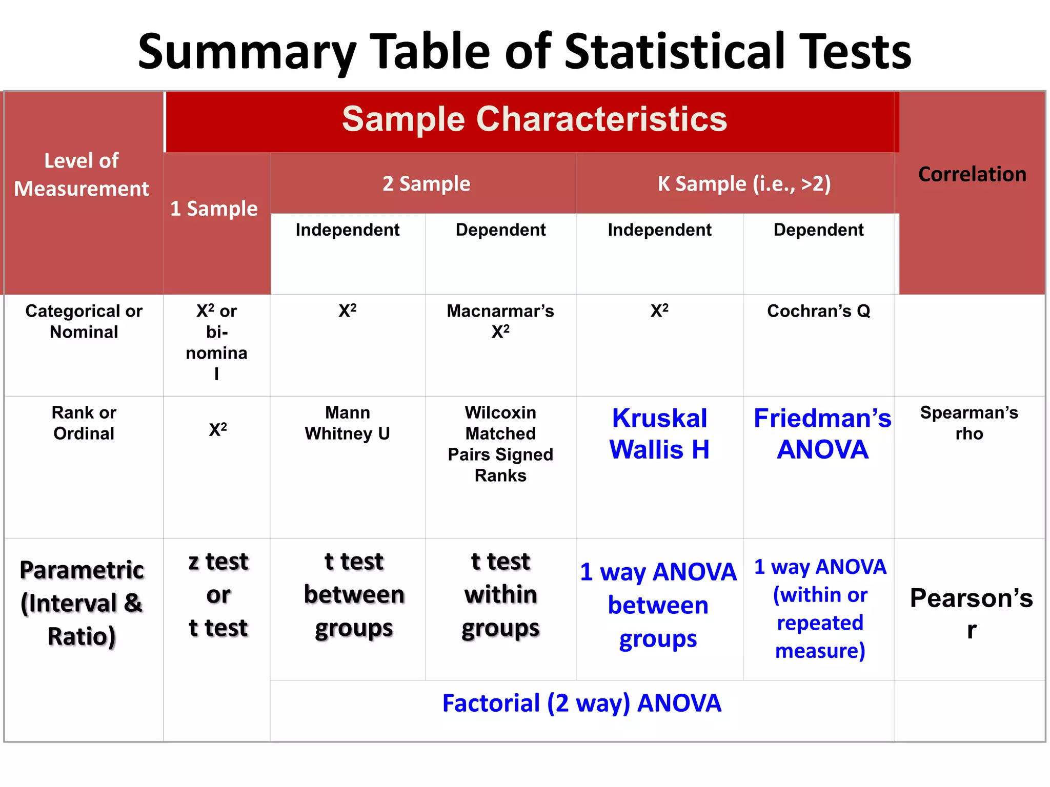
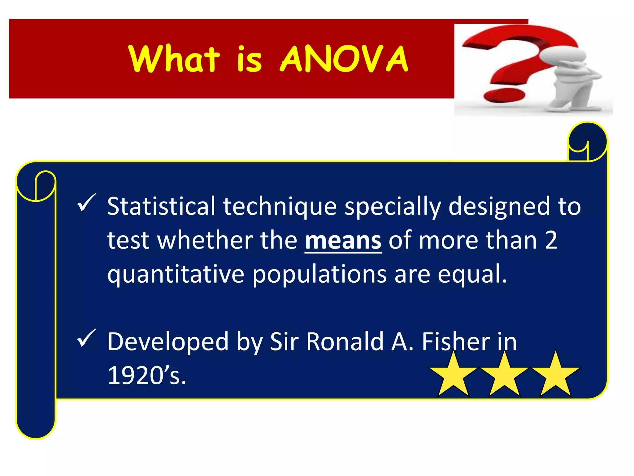
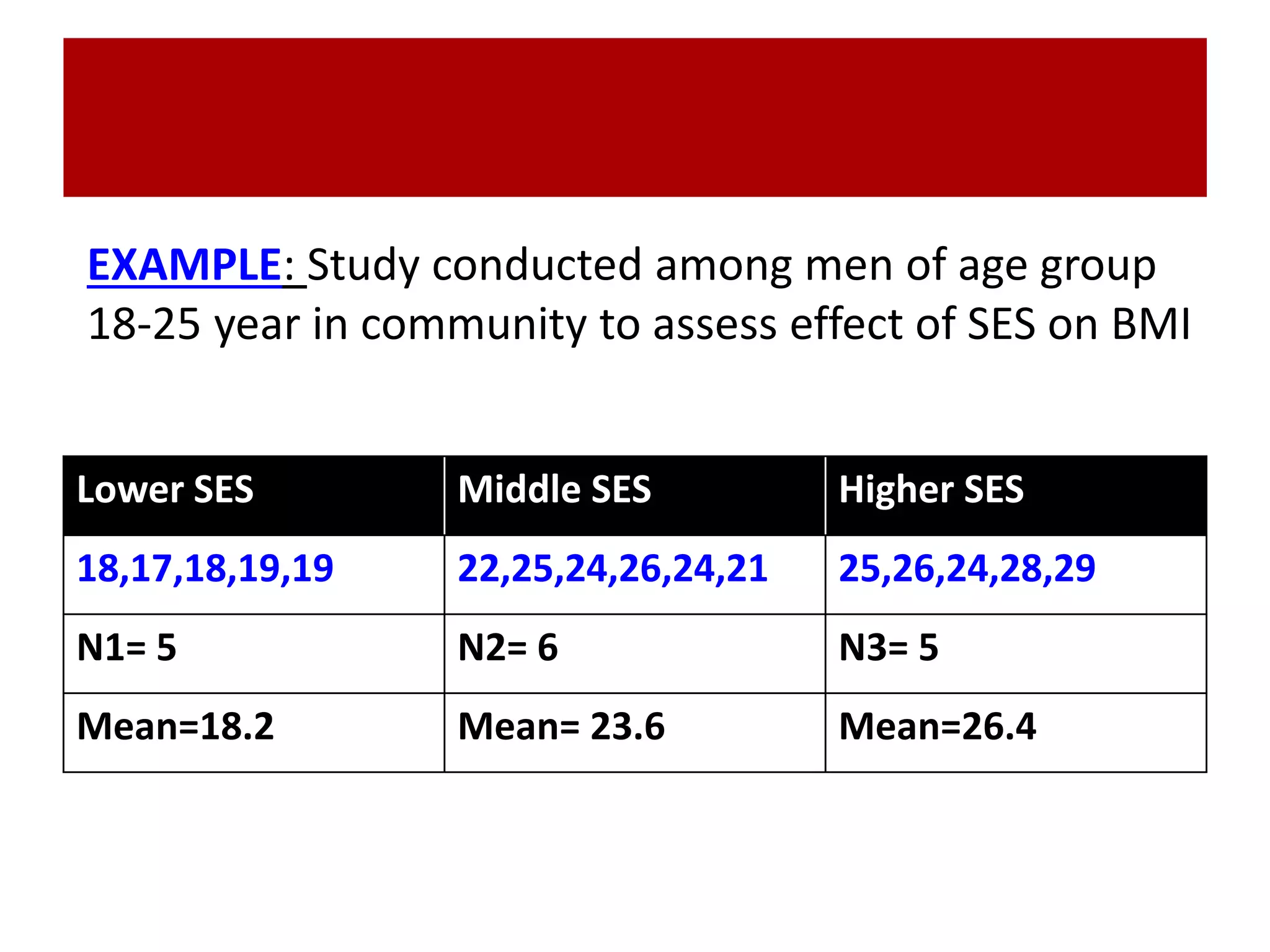
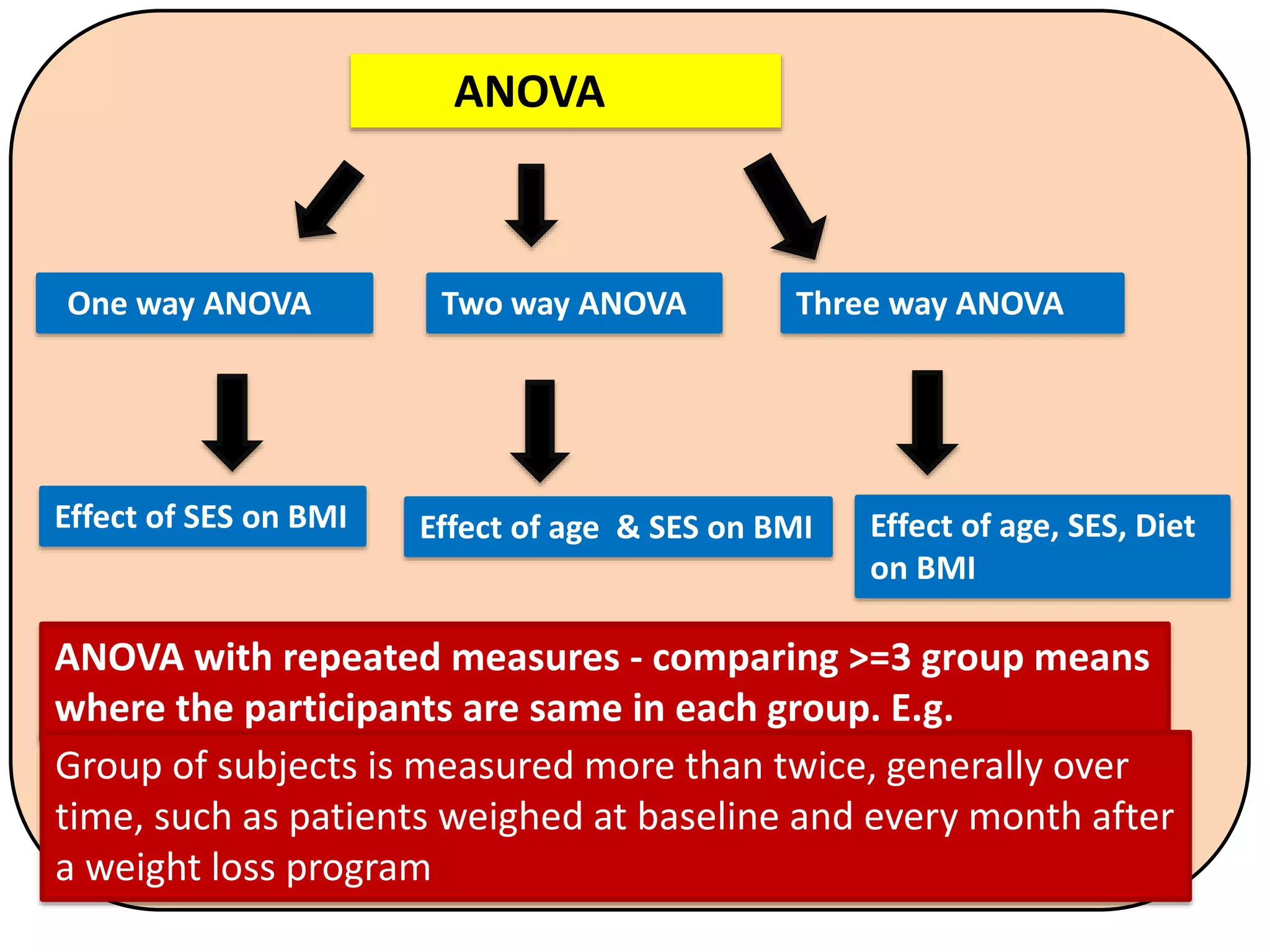
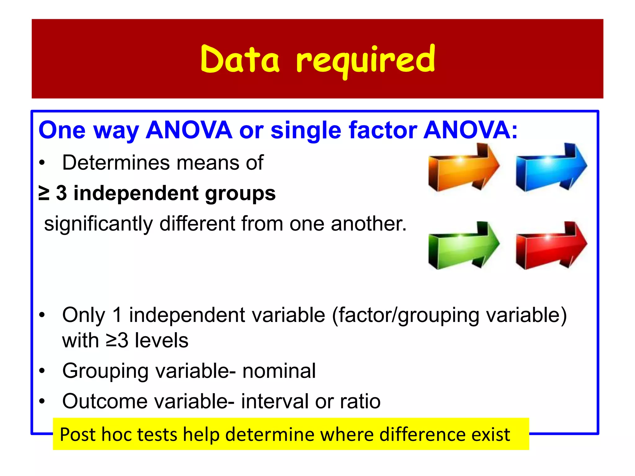
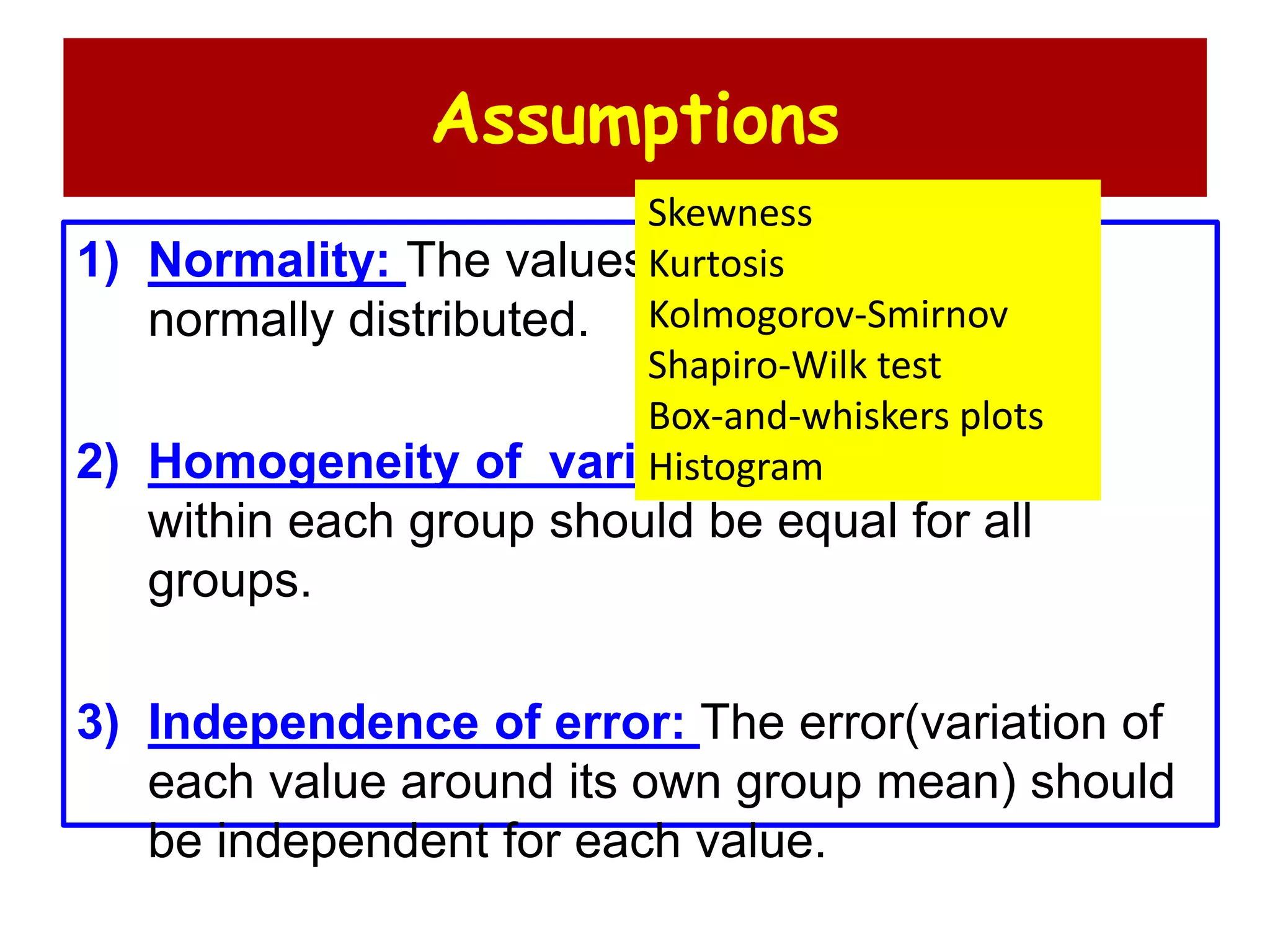
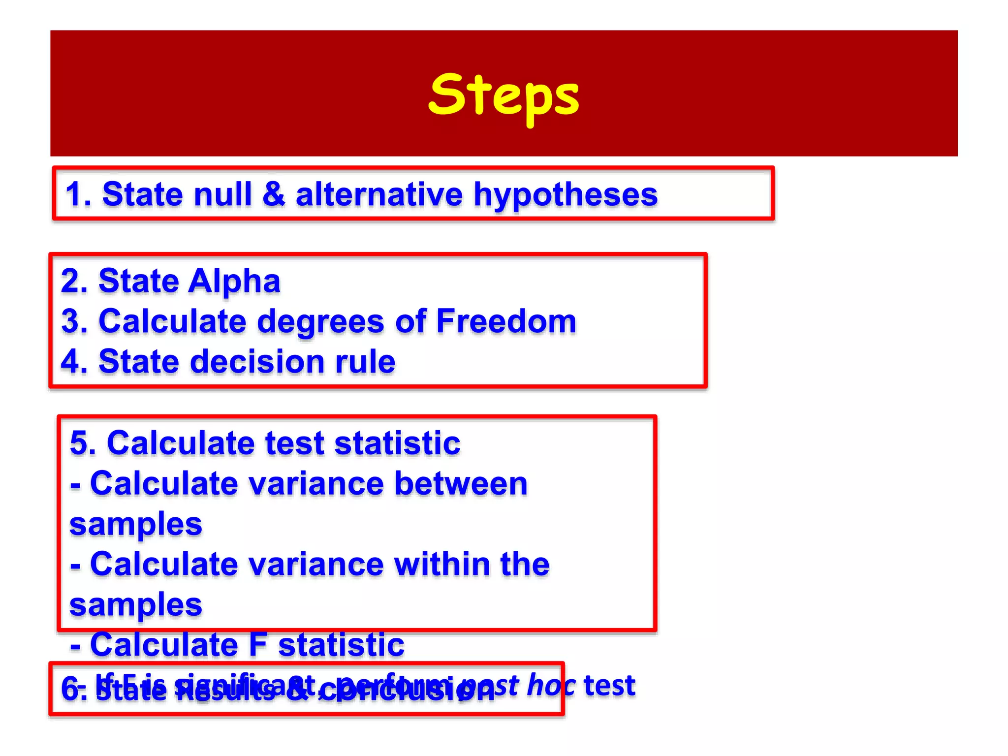
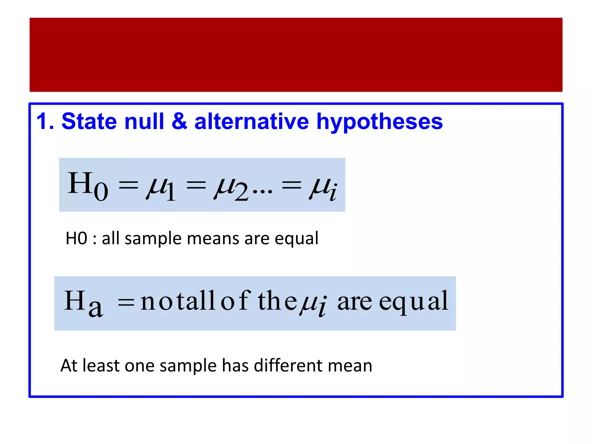
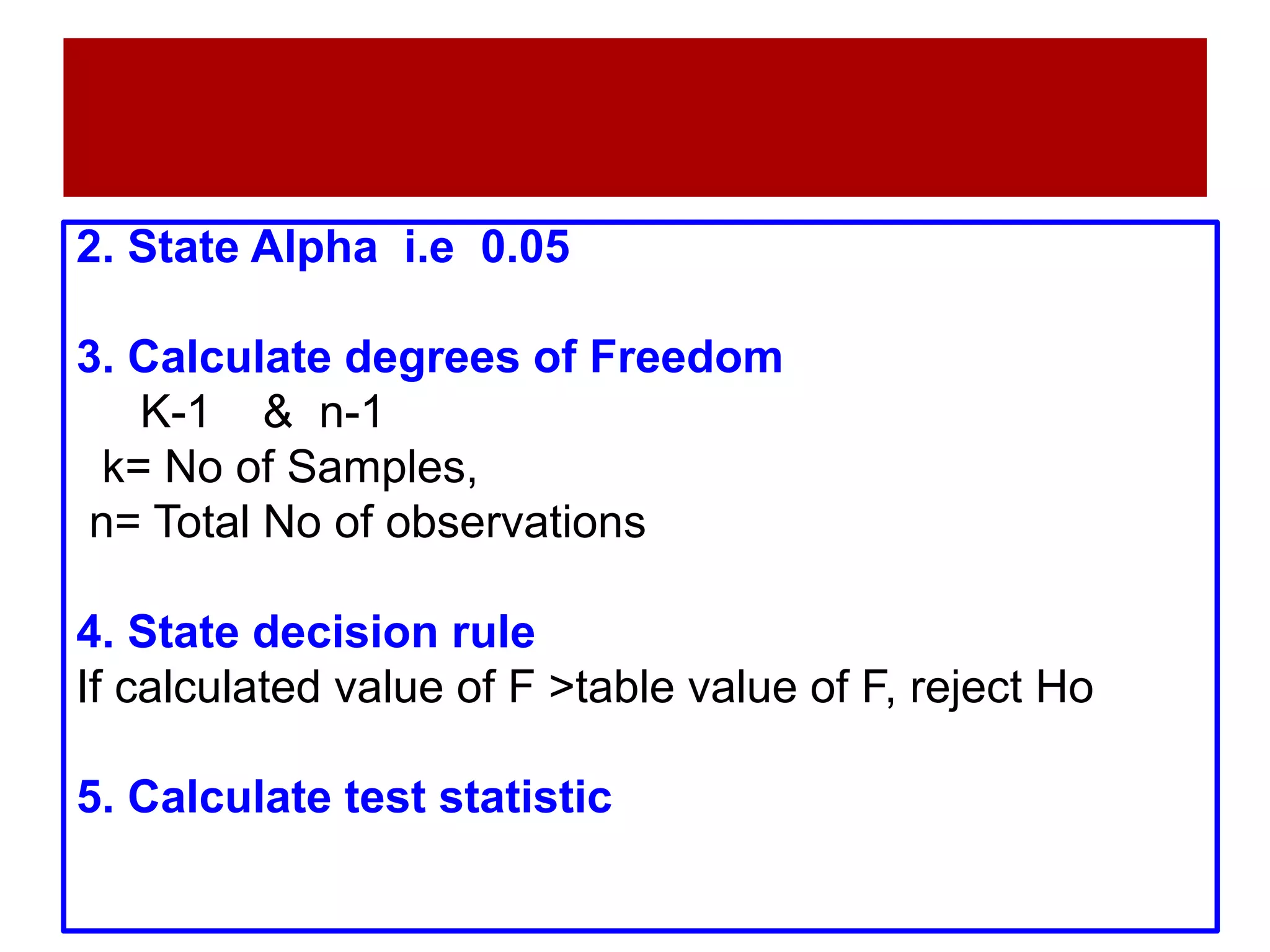
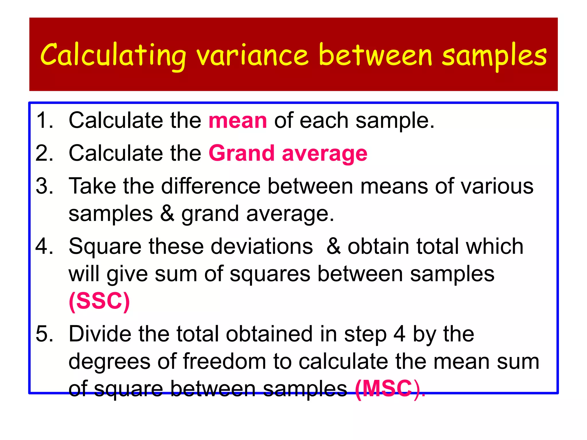
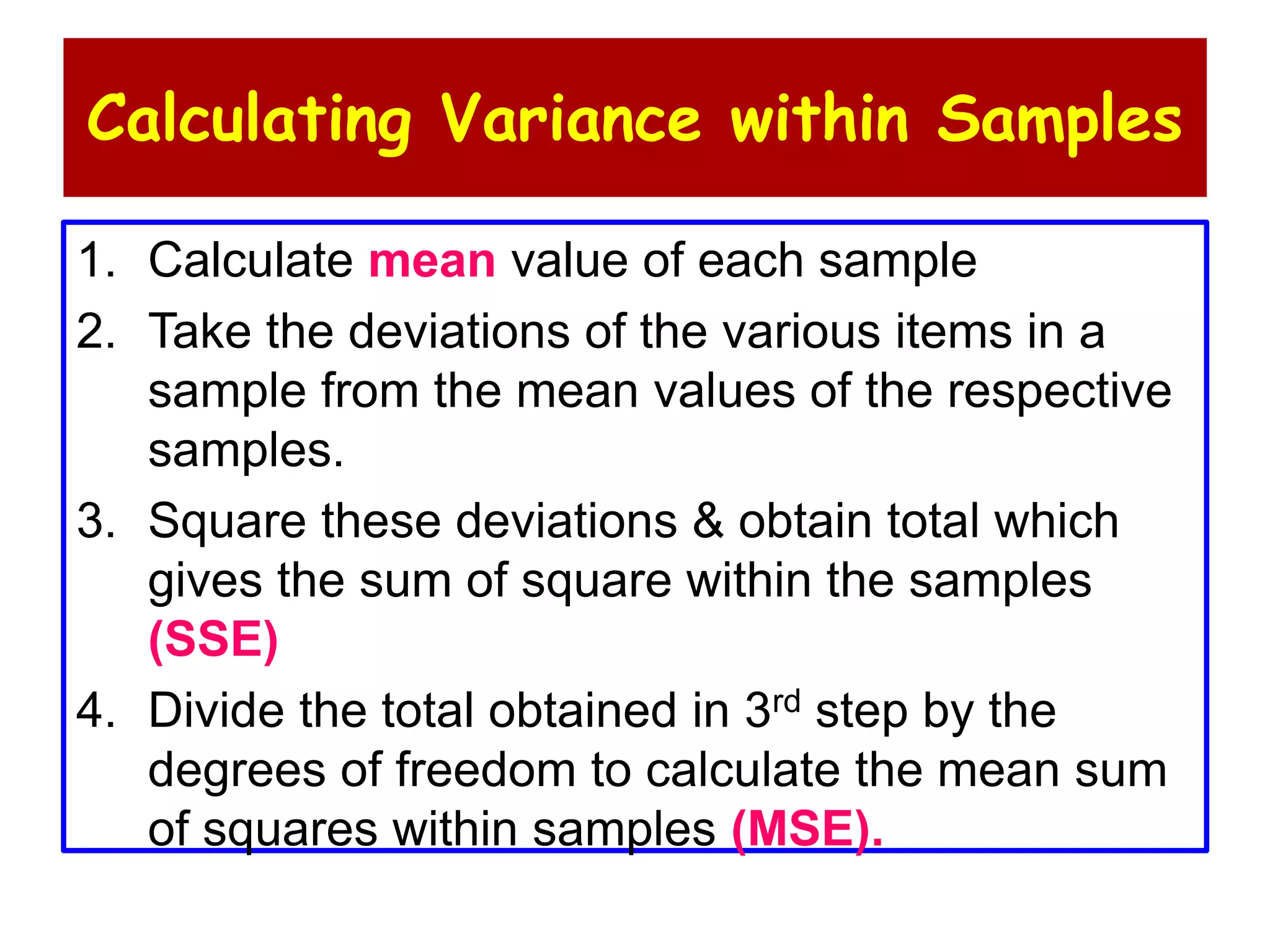
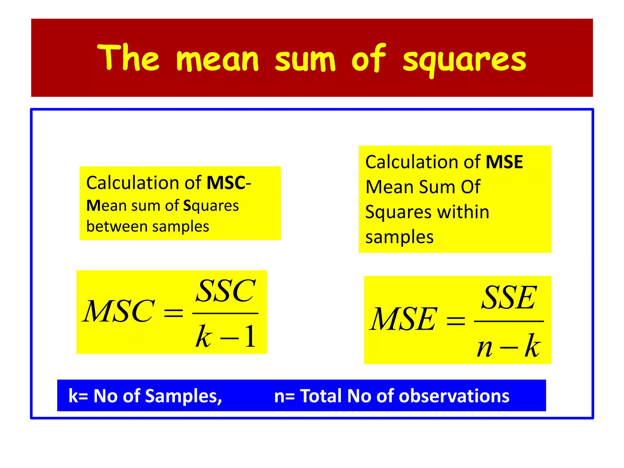
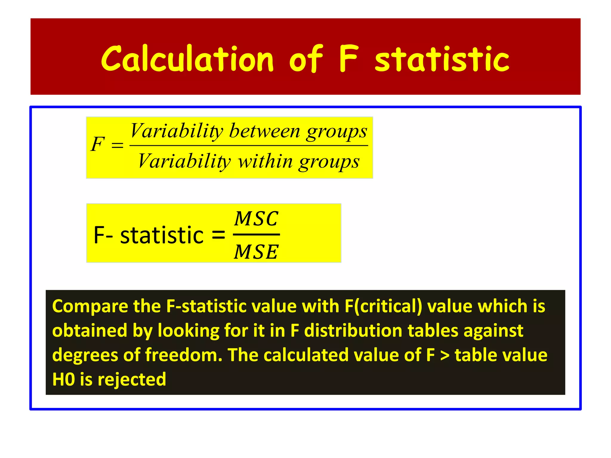
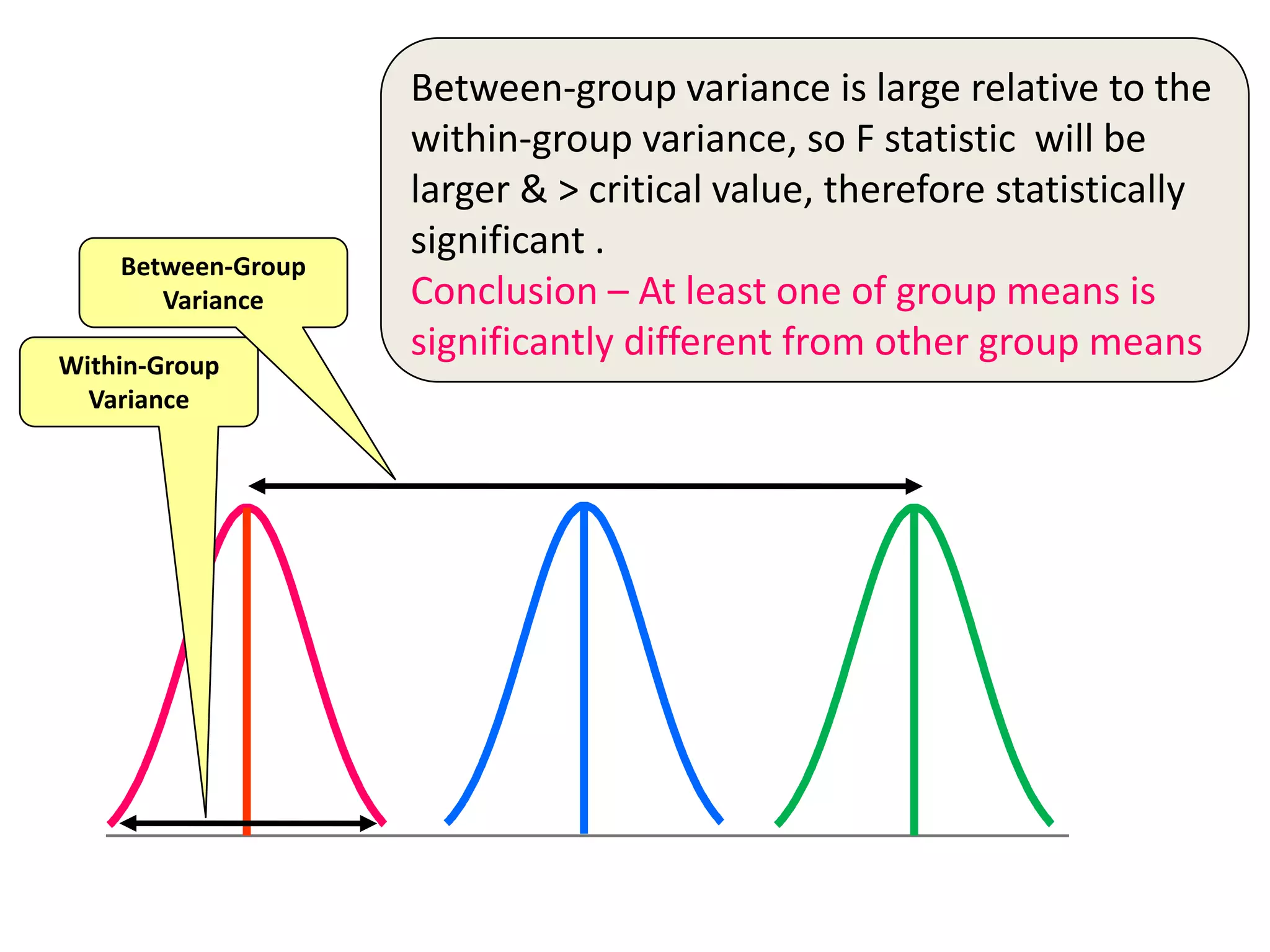
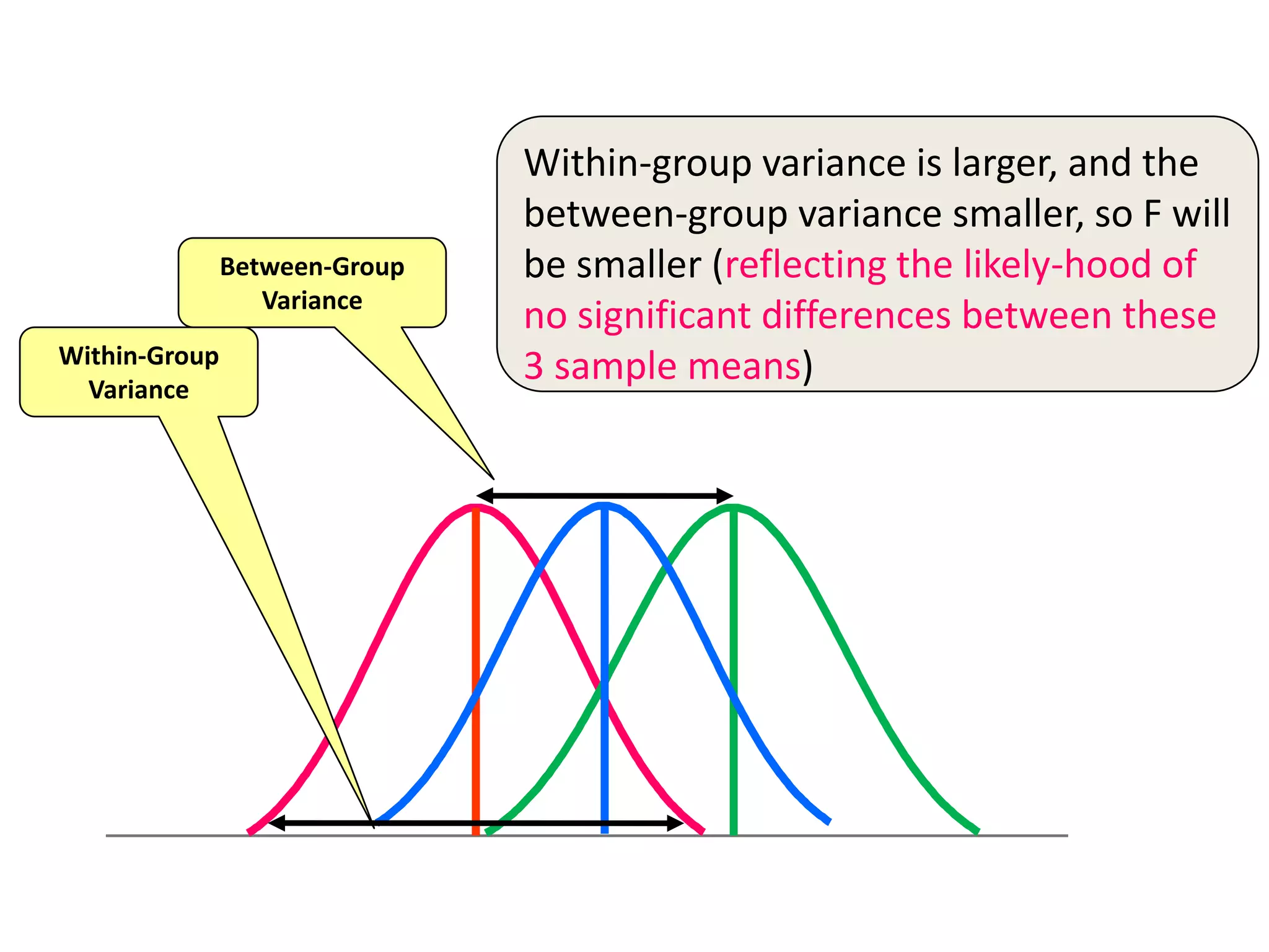
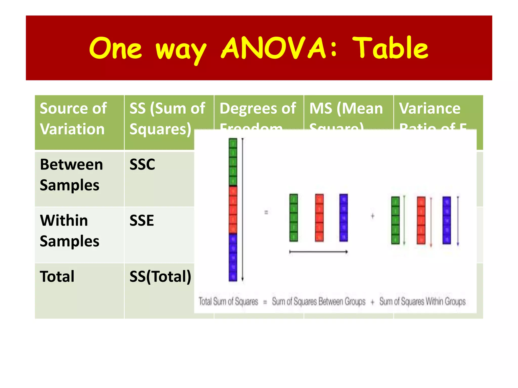
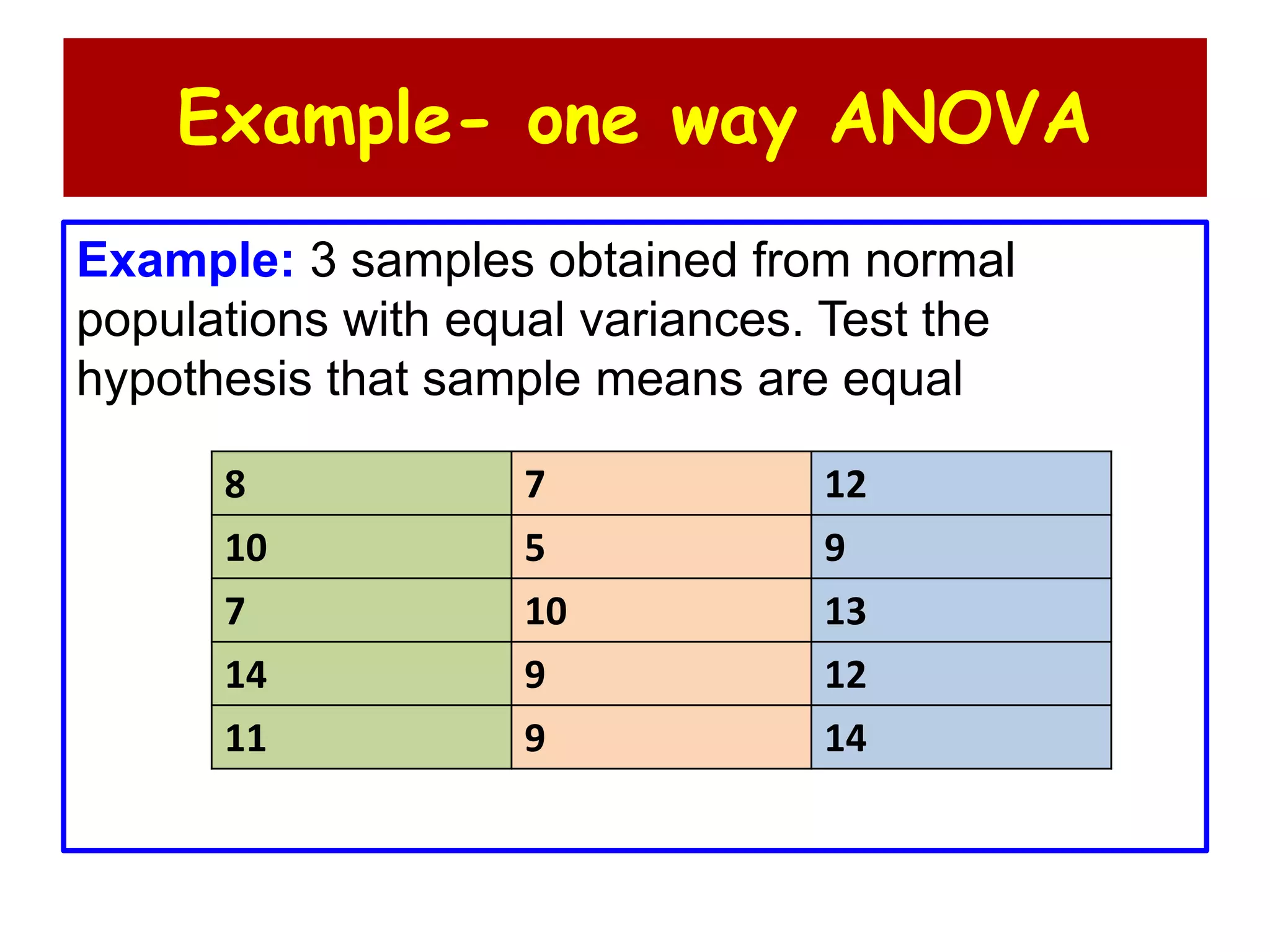
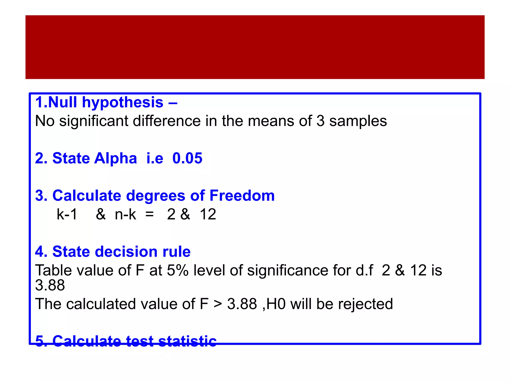
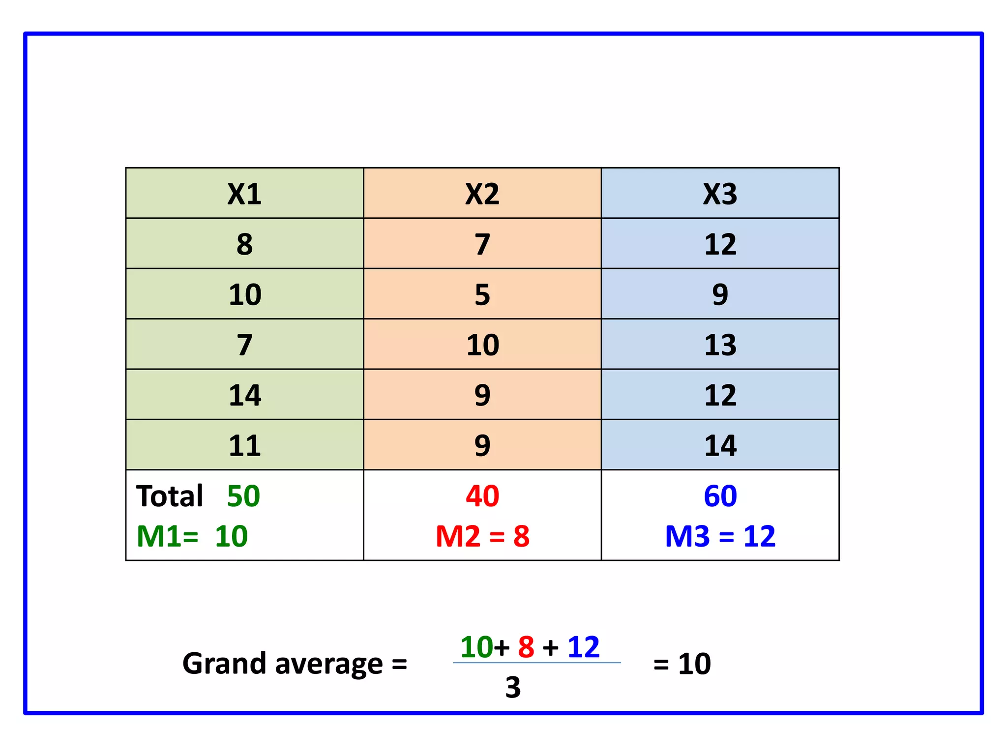
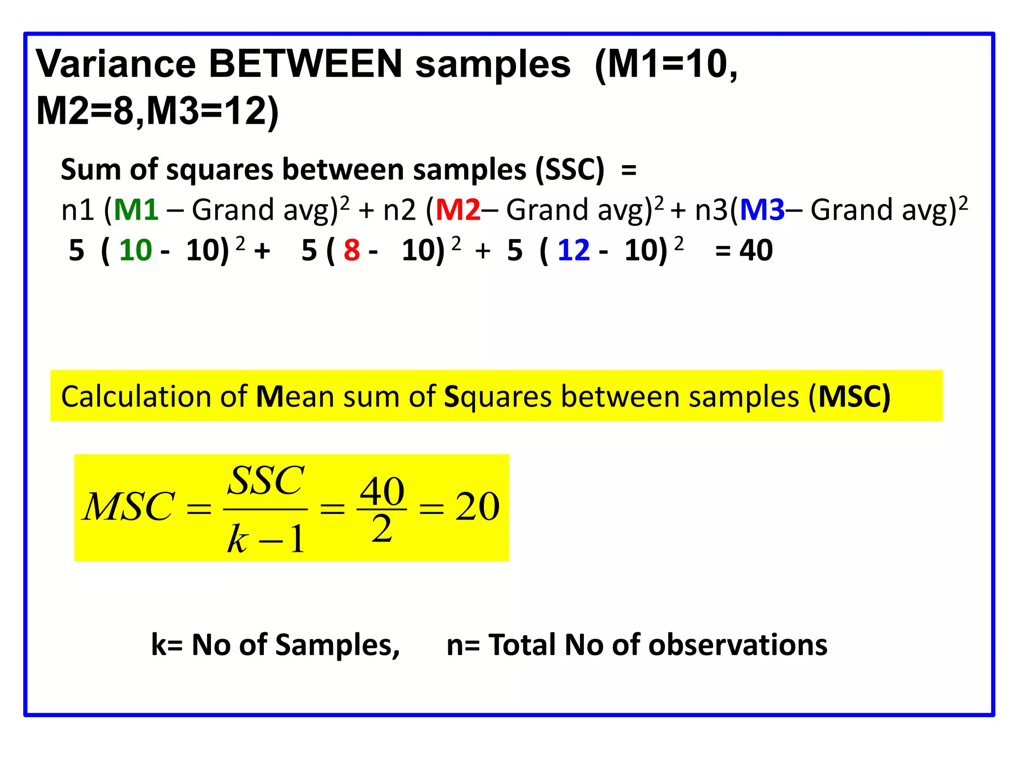
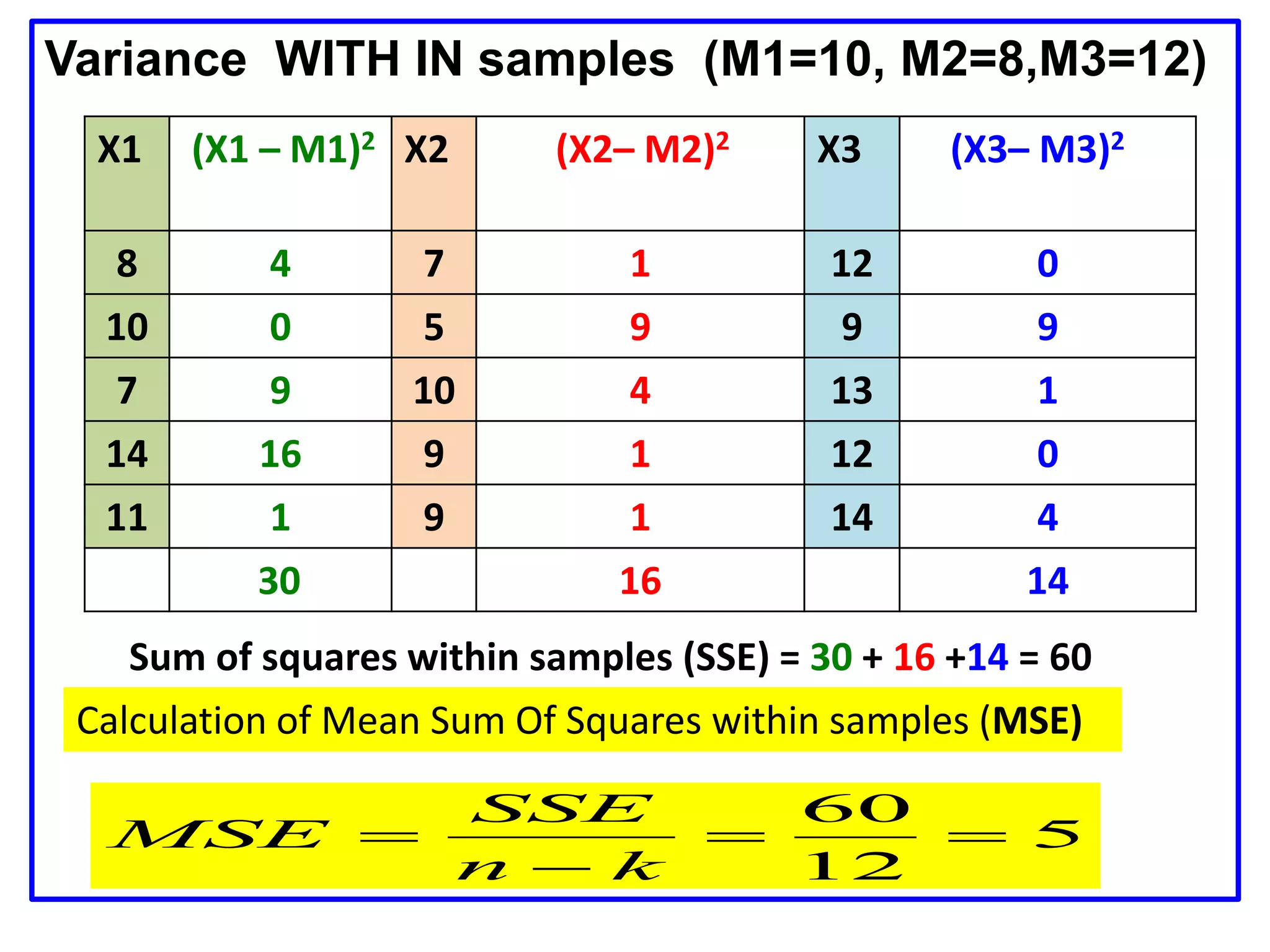
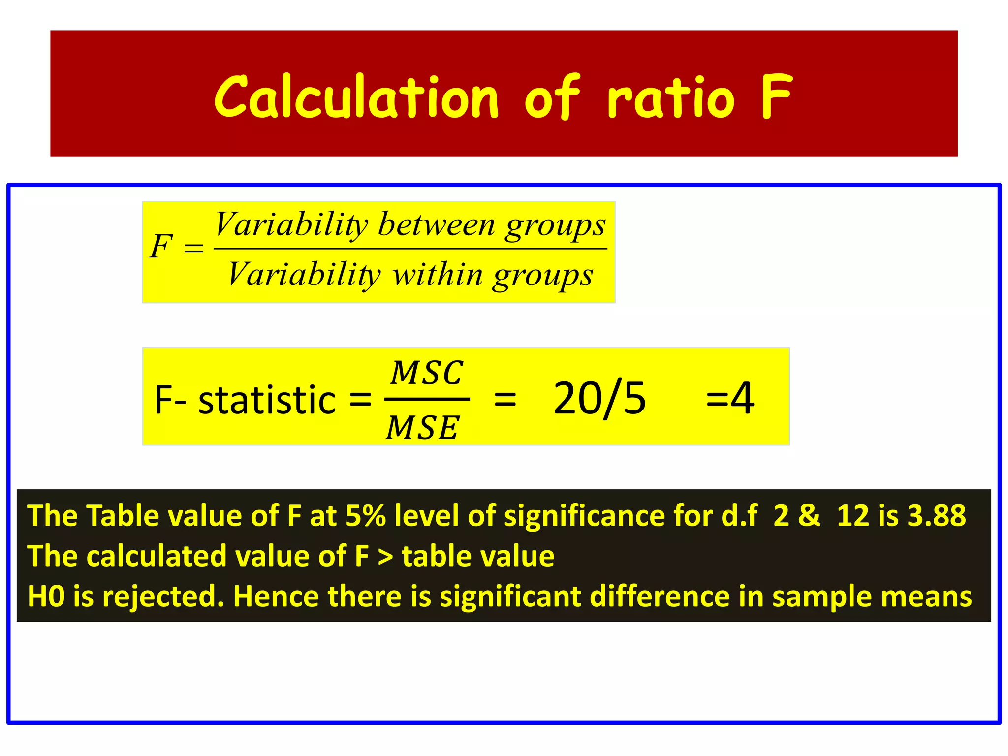
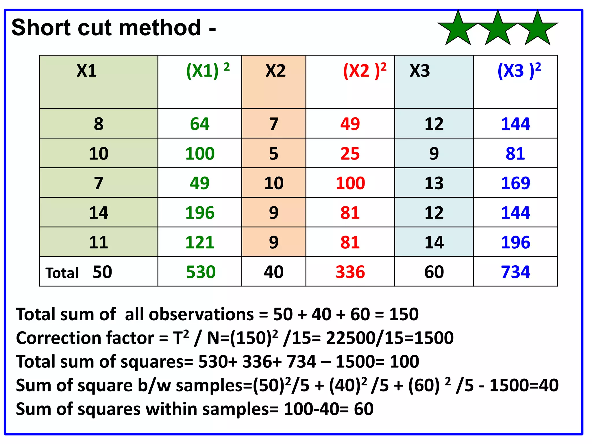
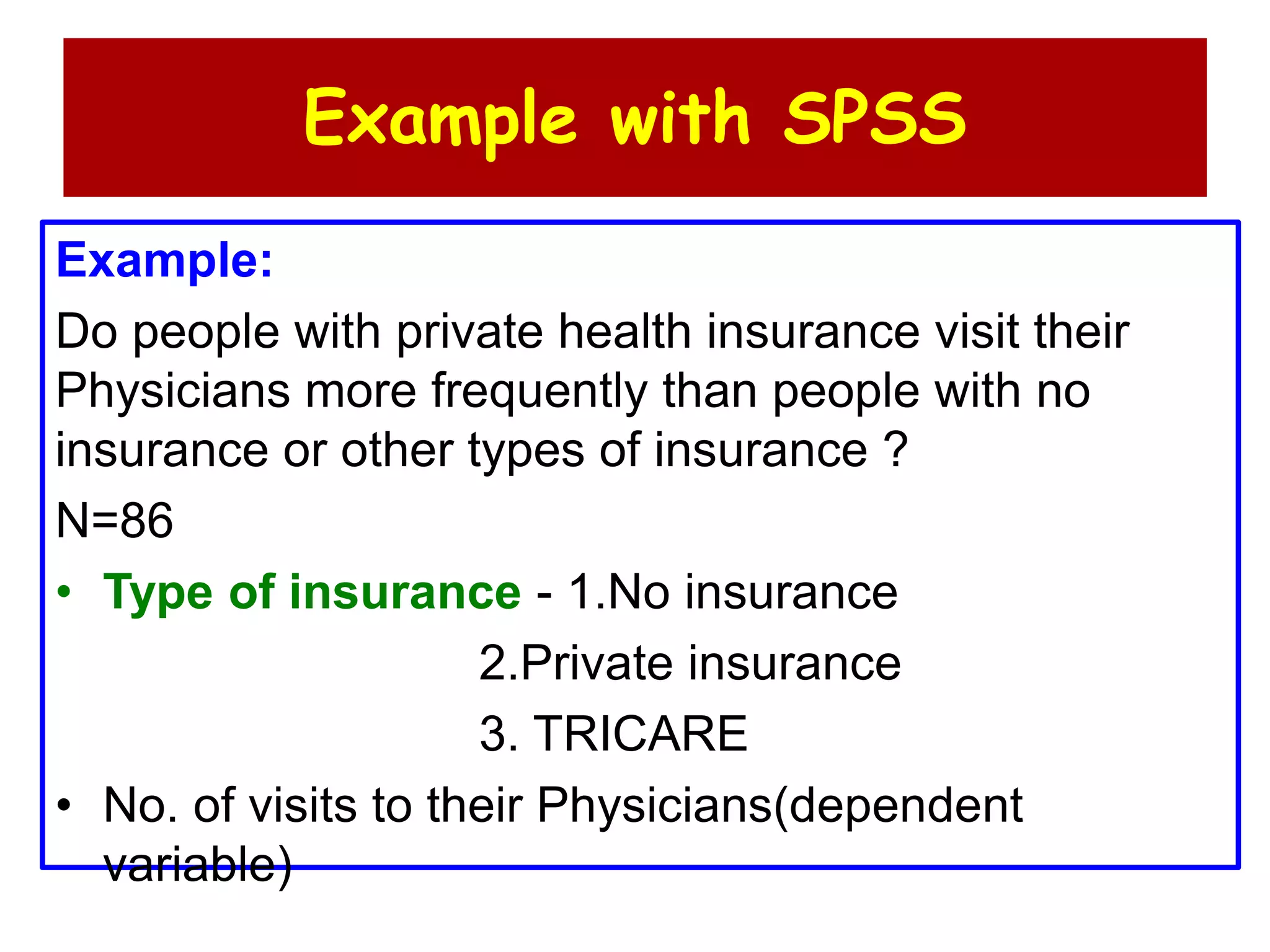
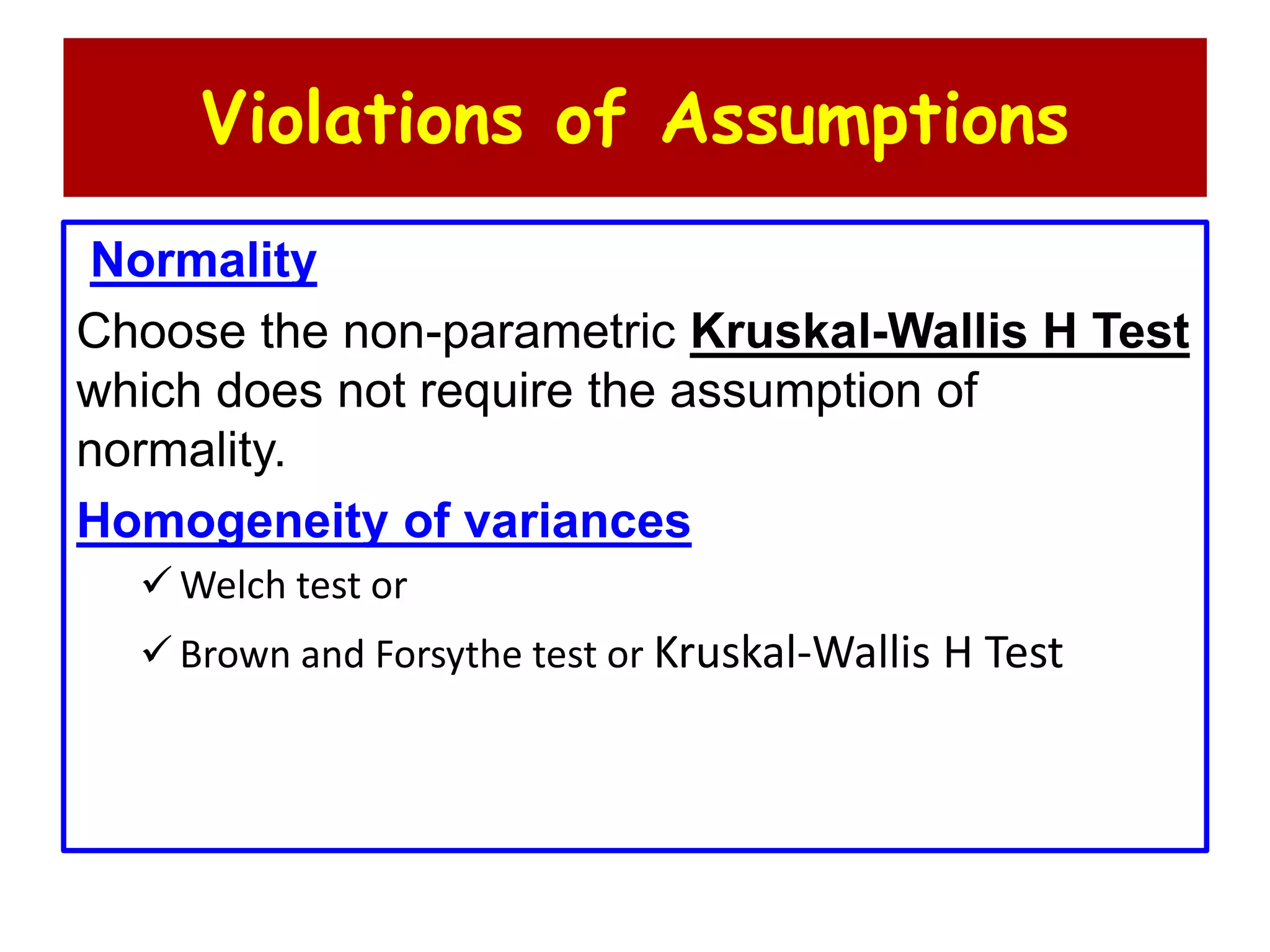

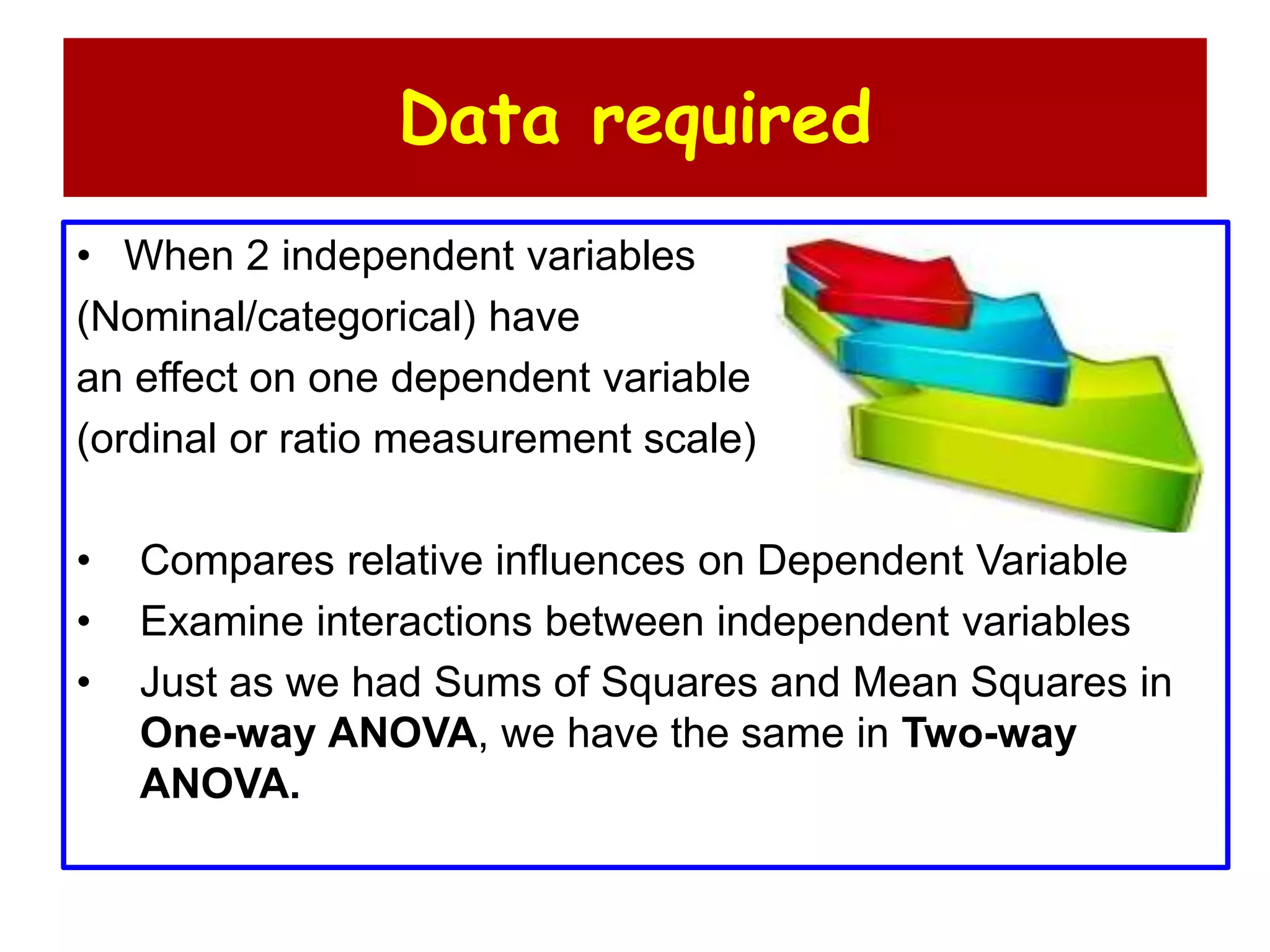
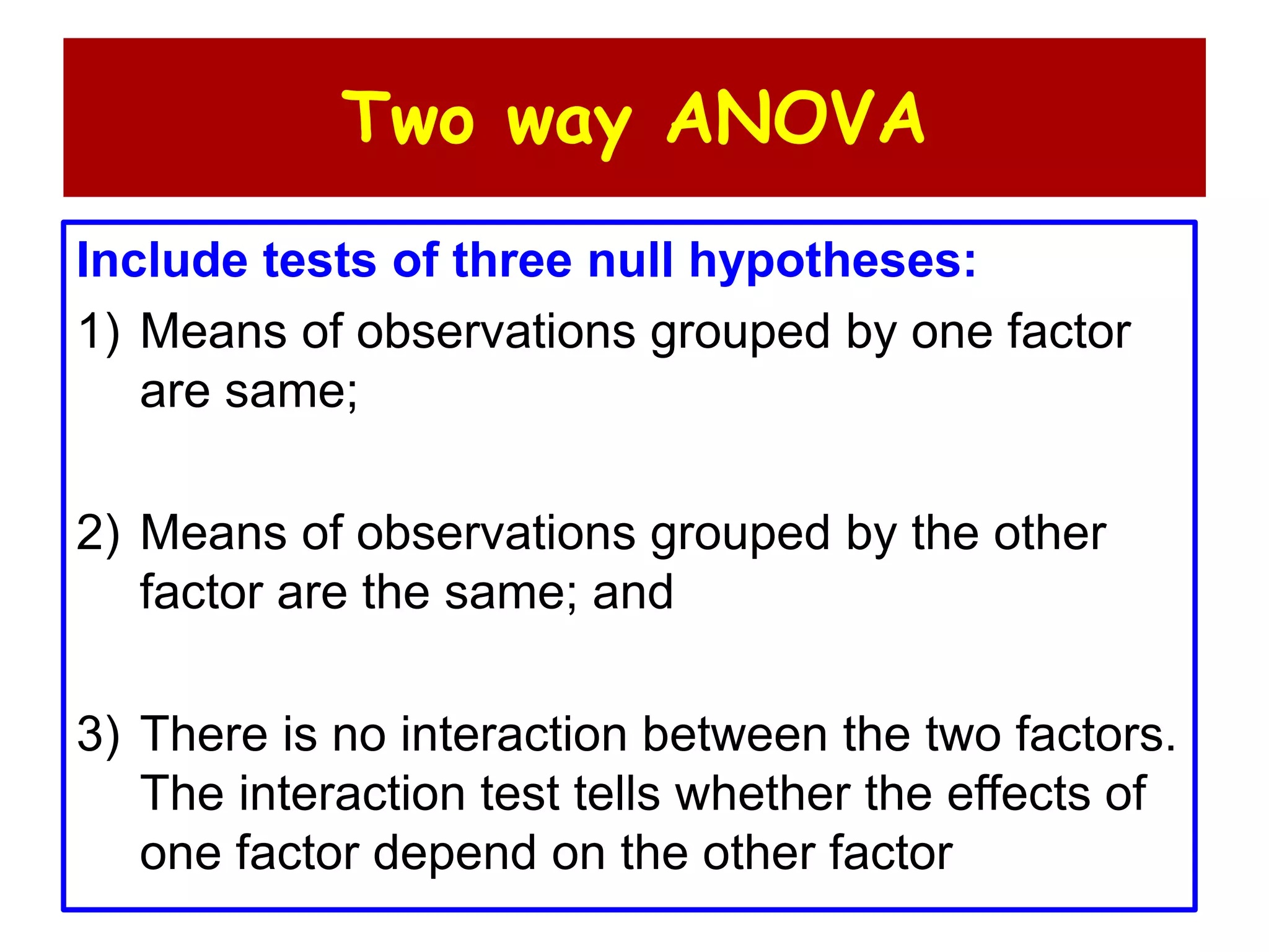
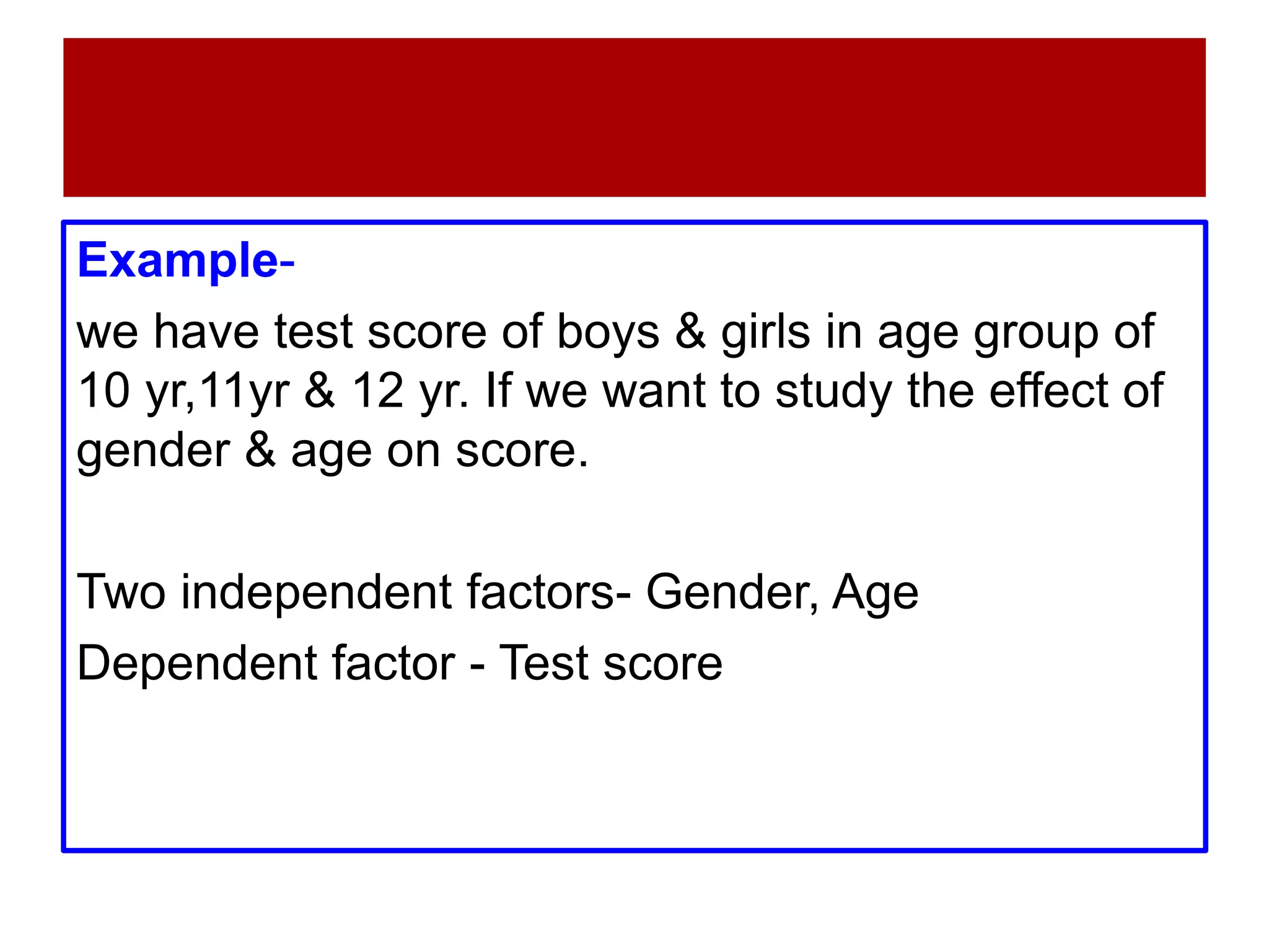
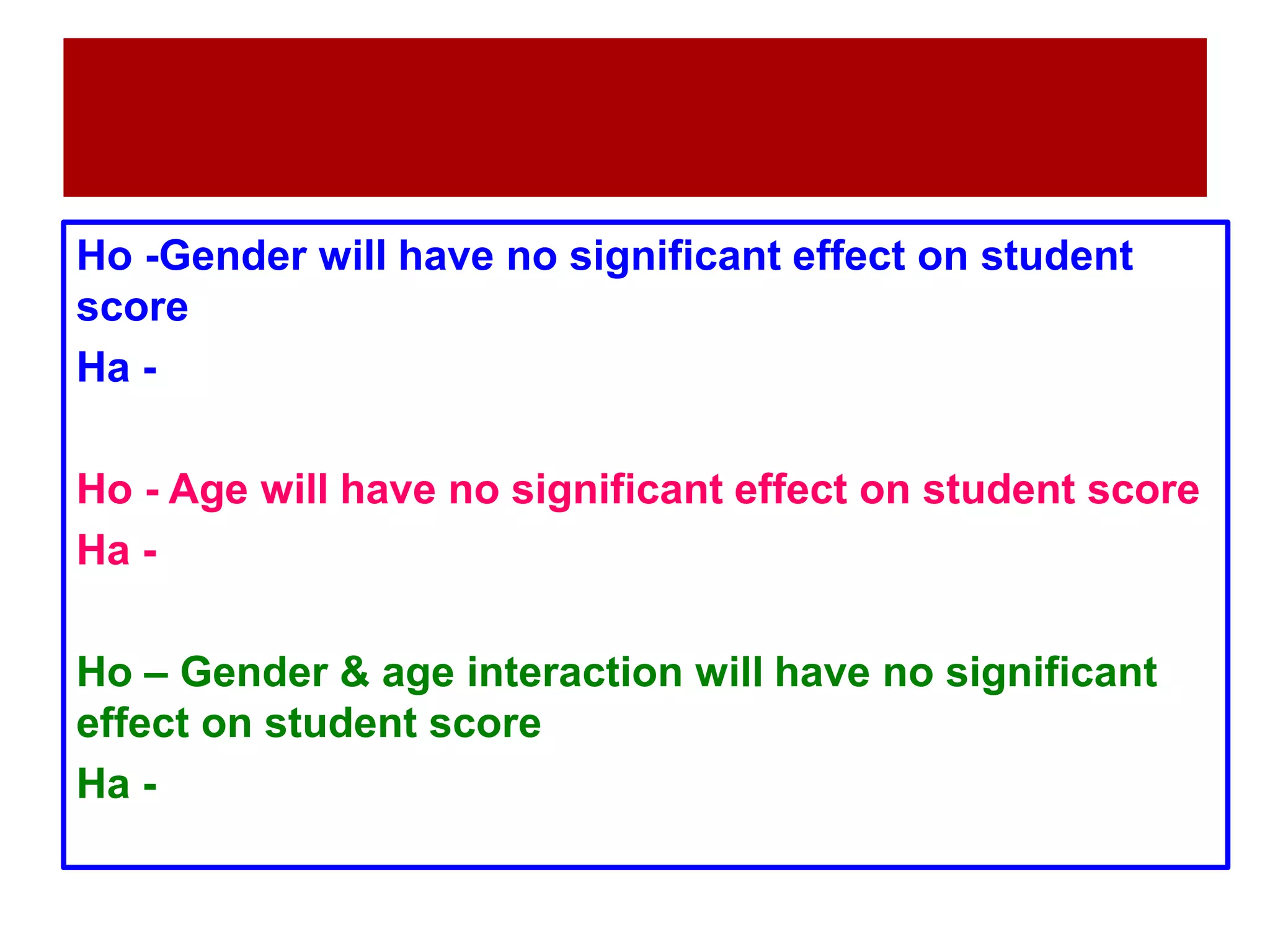
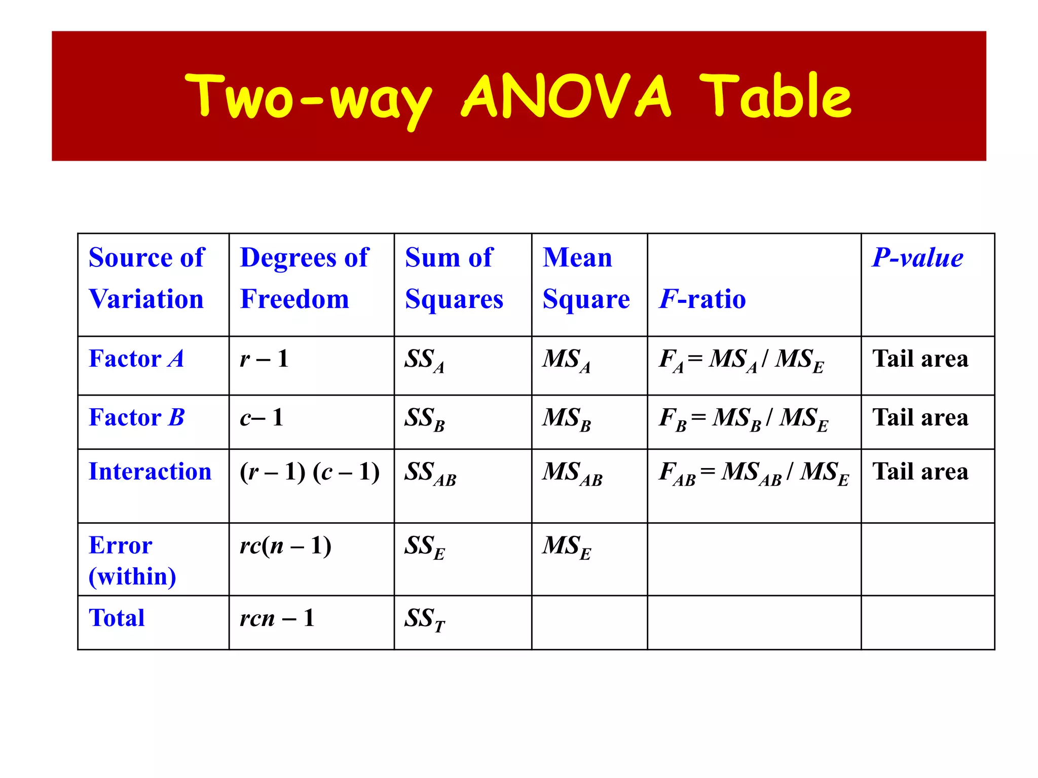
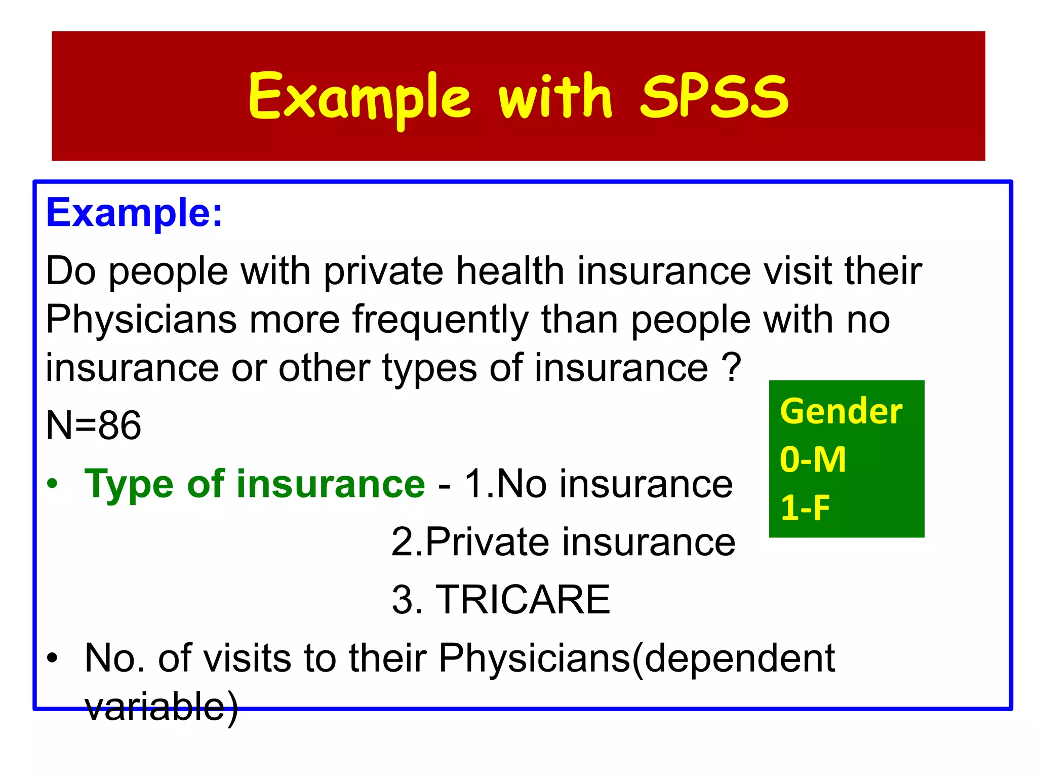

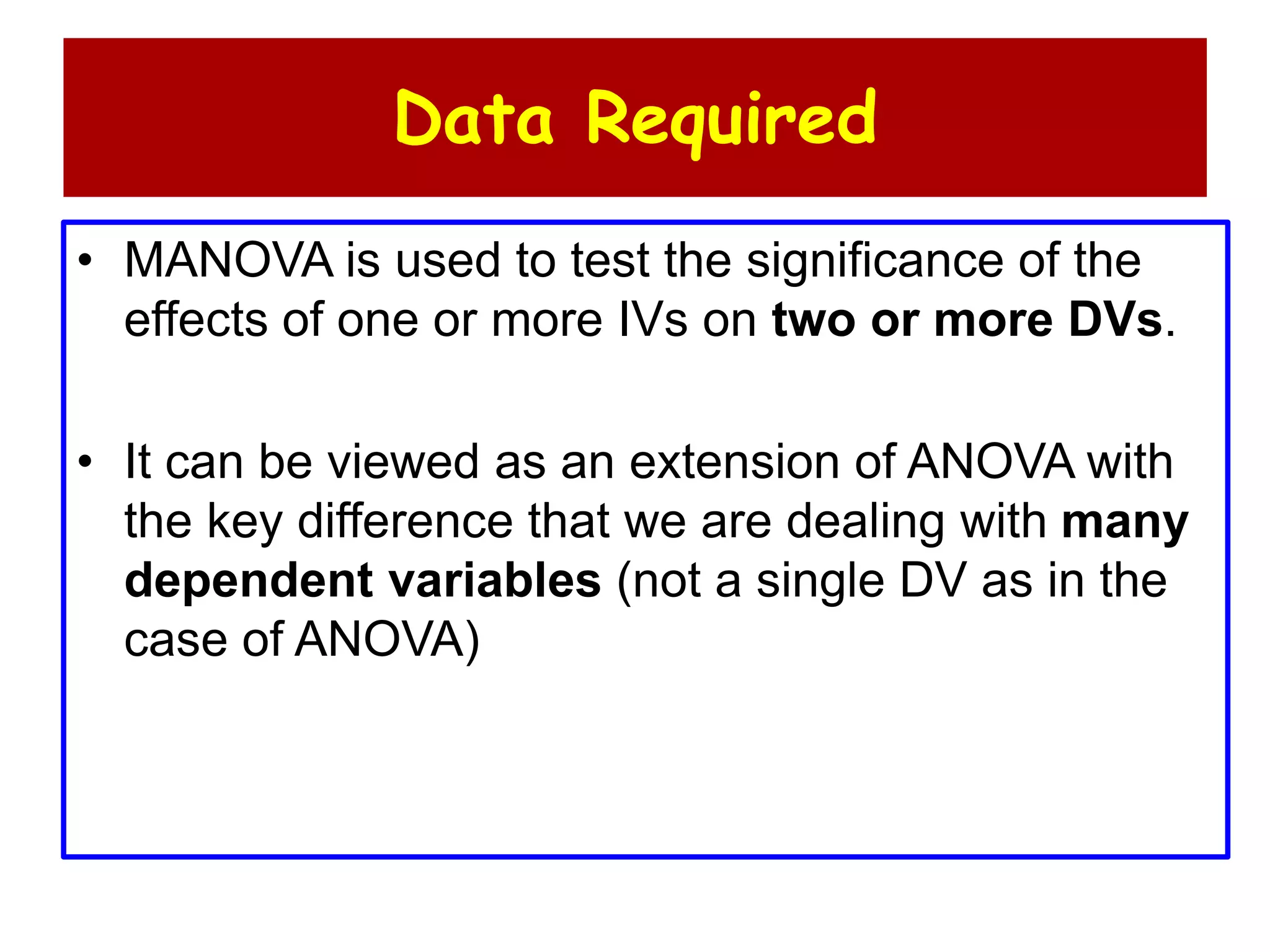

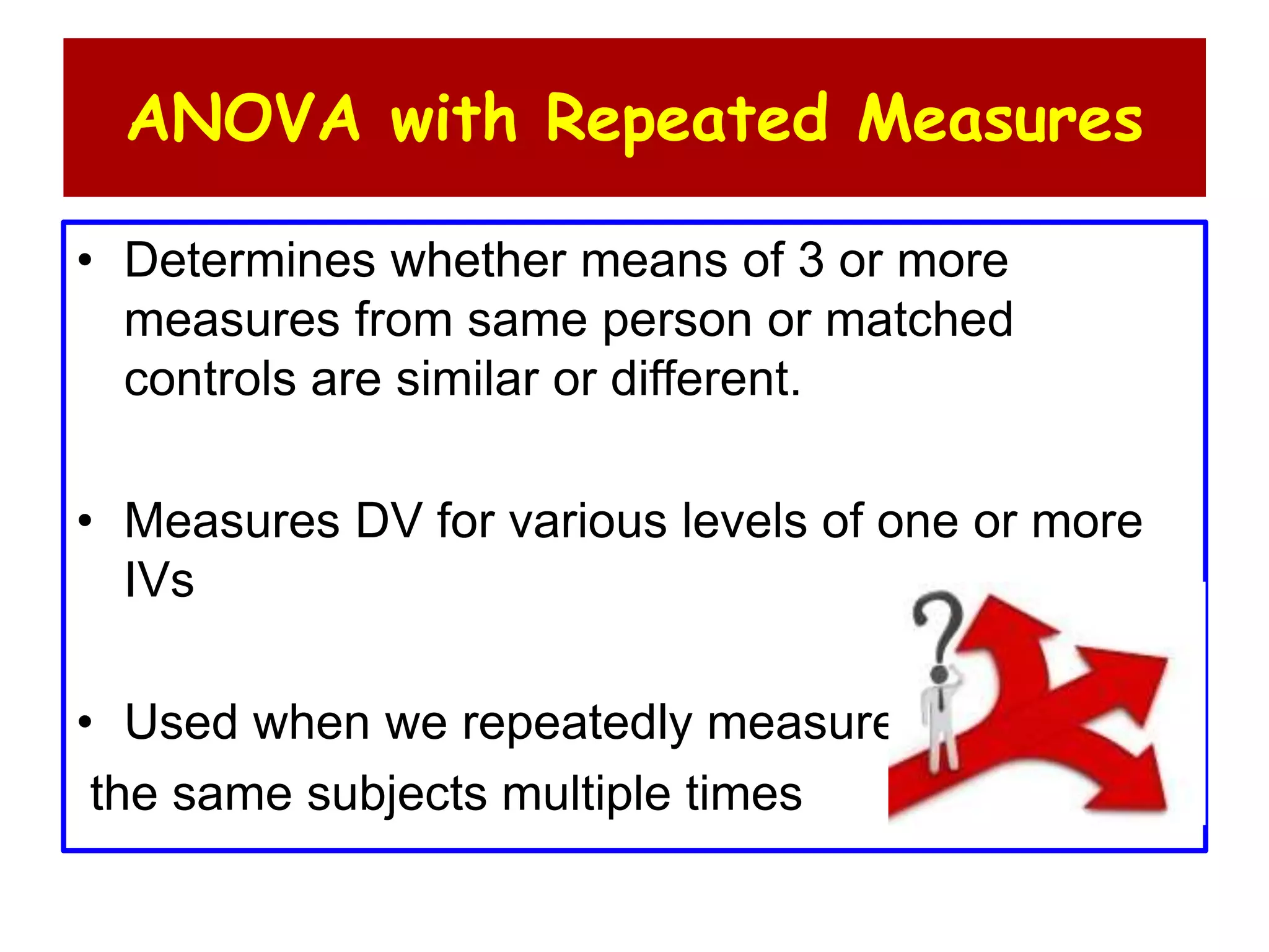
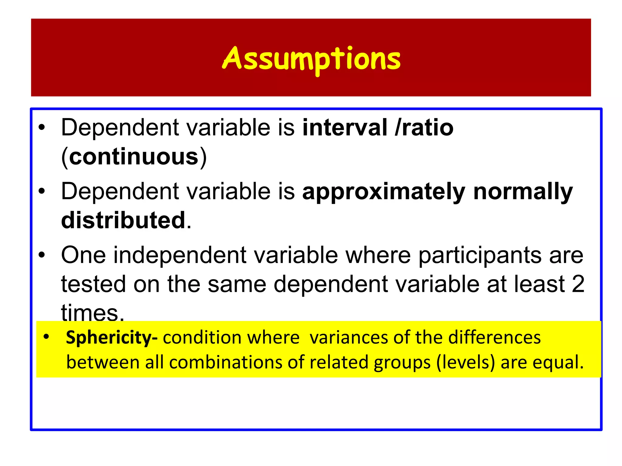
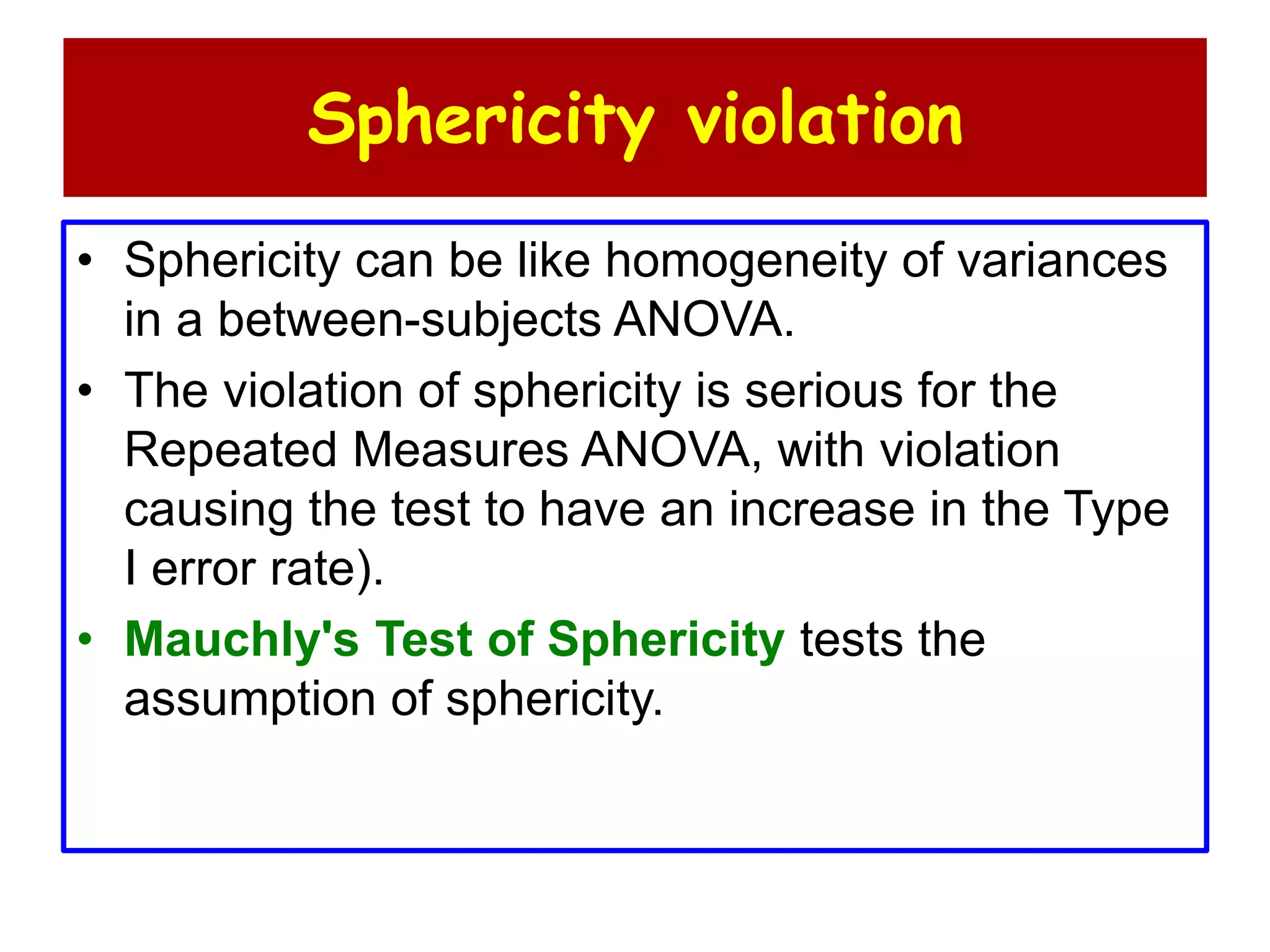
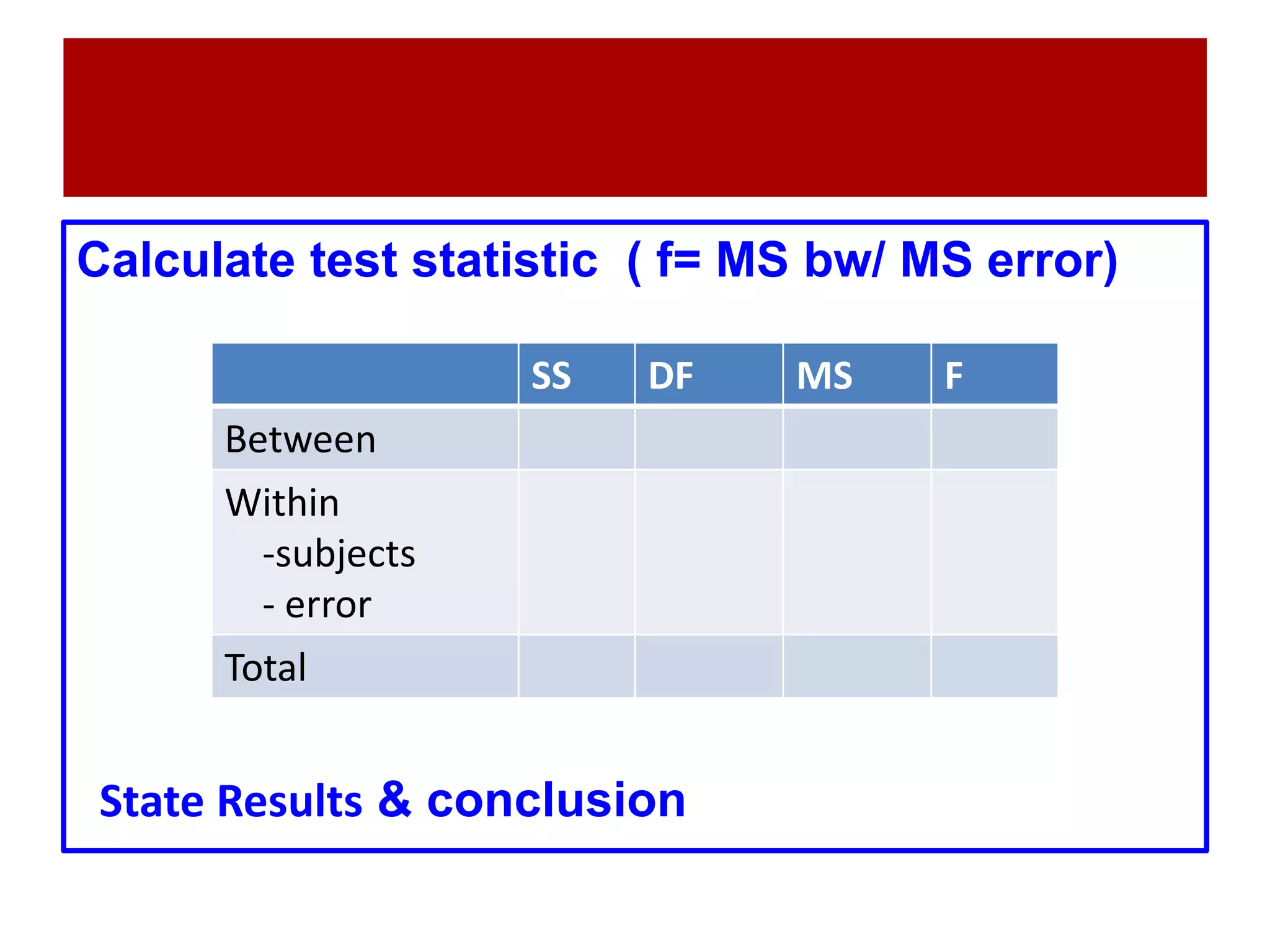
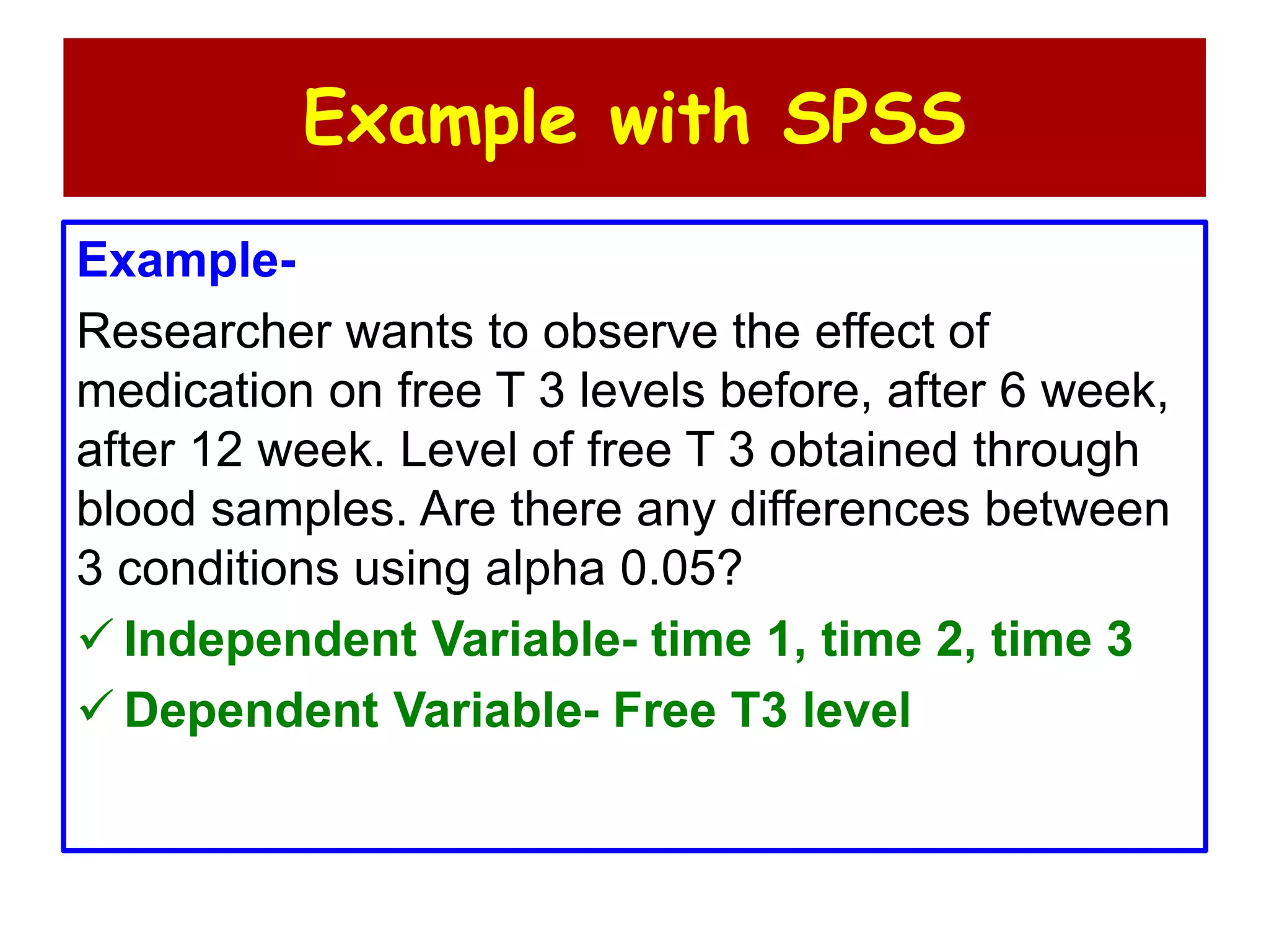
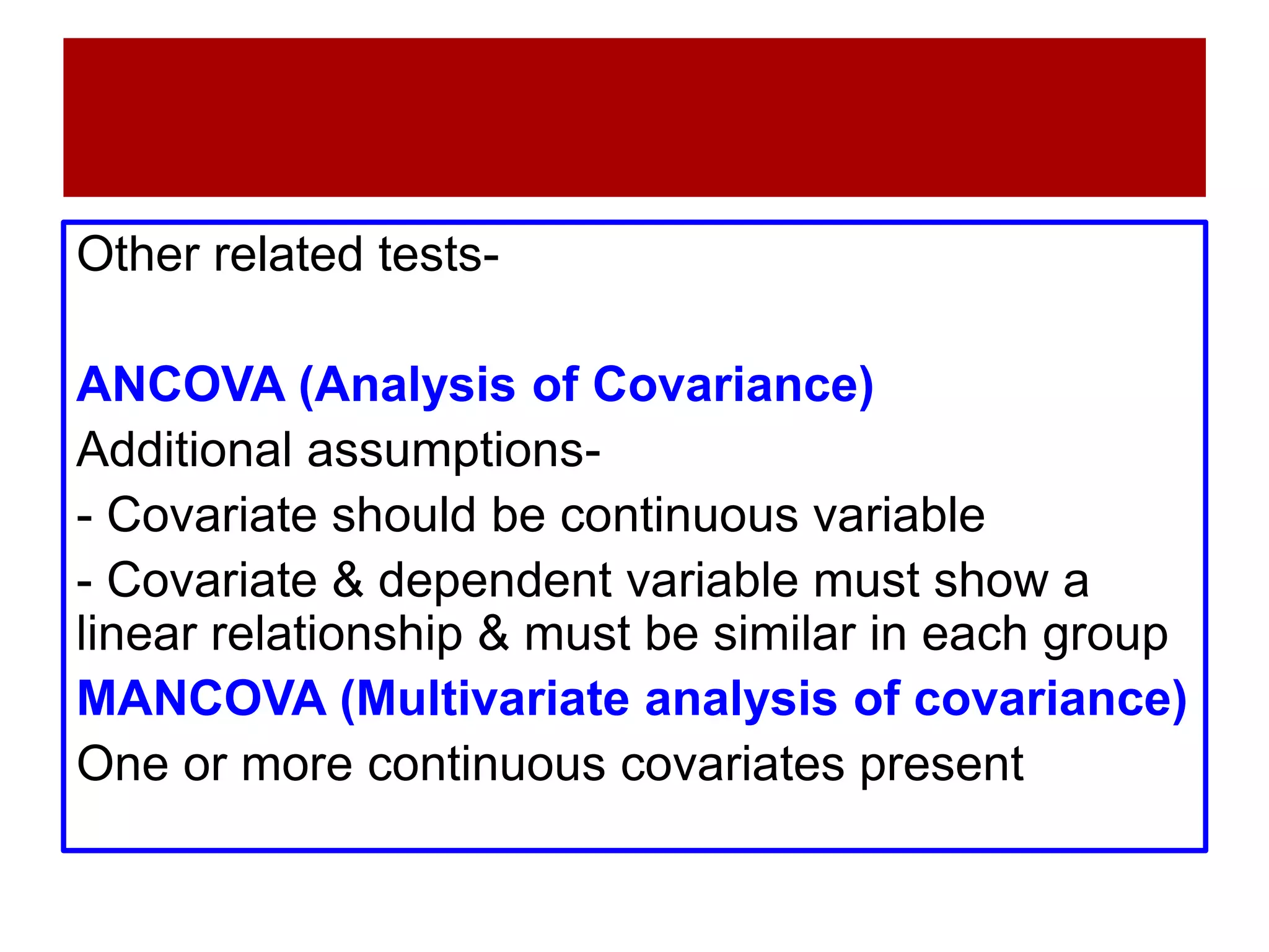


This document discusses various types of analysis of variance (ANOVA) statistical tests. It begins with an introduction to one-way ANOVA for comparing the means of three or more independent groups. Requirements for one-way ANOVA include a nominal independent variable with three or more levels and a continuous dependent variable. Assumptions of one-way ANOVA include normality and homogeneity of variances. The document then briefly discusses two-way ANOVA, MANOVA, ANOVA with repeated measures, and related statistical tests. Examples of each type of ANOVA are provided.


![[DSC Europe 25] Joseph Marks - From Ledgers To Transformers: How AI & Cloud A...](https://cdn.slidesharecdn.com/ss_thumbnails/11yfjb86tpcpsh9yqg4c-8-251128093135-7ad97865-thumbnail.jpg?width=640&height=640&fit=bounds)
![[DSC Europe 25] Stefan_Milosevic - AI and digital twins in precision oncology...](https://cdn.slidesharecdn.com/ss_thumbnails/nnmuciuxr2ugh4d9pzkg-1-251126104228-148c7fe8-thumbnail.jpg?width=640&height=640&fit=bounds)
![[DSC Europe 25] Milan Misic - RAG, recommenders and face recognition applica...](https://cdn.slidesharecdn.com/ss_thumbnails/mxe0wzfeqkortbfecopo-8-251128093135-51a402bb-thumbnail.jpg?width=640&height=640&fit=bounds)


![[DSC Europe 25] Jurij Kodre - What Can Healthcare Learn From Finance.pptx](https://cdn.slidesharecdn.com/ss_thumbnails/q87nzrwtd6ihsqqtrqdr-7-251126104228-00657fba-thumbnail.jpg?width=640&height=640&fit=bounds)


