VVB_DWM Module no 2_Data exploration and data preprocessing .pptx
this is module to of data in mining and scratty Vashi computer science in engineering so this covers various topics like data exploration and data preprocessing
VVB_DWM Module no 2_Data exploration and data preprocessing .pptx
1.
Module No :02
Data Exploration & Data Preprocessing
1
2.
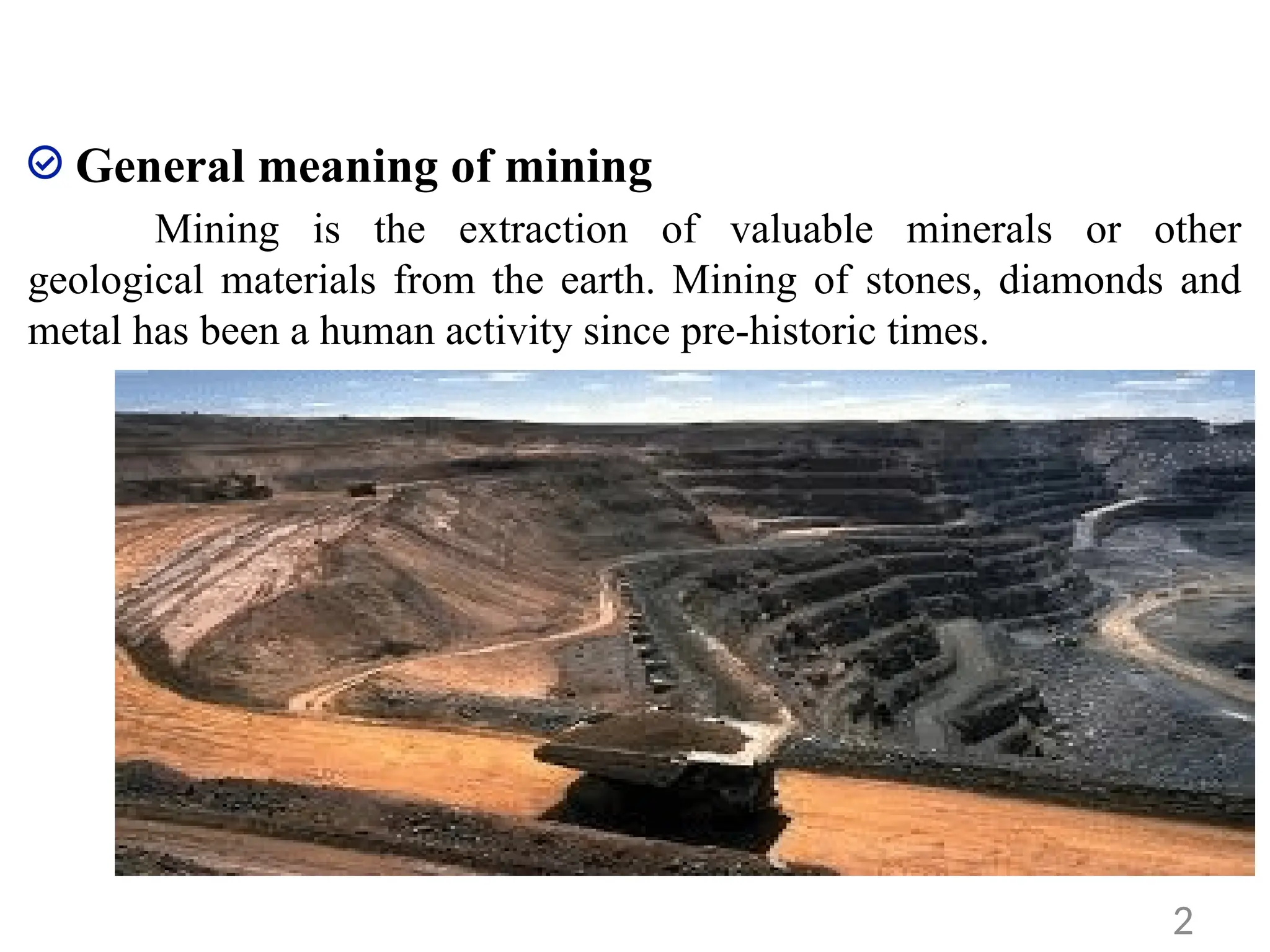
General meaning ofmining
Mining is the extraction of valuable minerals or other
geological materials from the earth. Mining of stones, diamonds and
metal has been a human activity since pre-historic times.
2
3.
What is DataMining? Non technical view
1. There are things that we know that we know…
2. There are things that we know that we don’t know…
3. There are things that we don’t know we don’t know.”
Data mining is not finding something it is all about
discovering
e.g. Columbus “discovered” America
3
4.
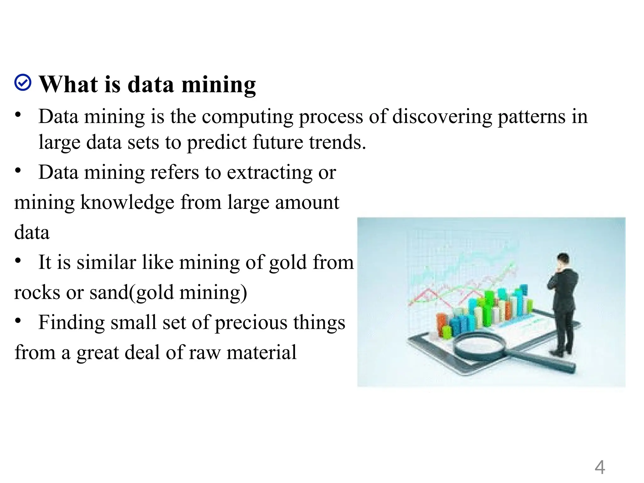
What is datamining
• Data mining is the computing process of discovering patterns in
large data sets to predict future trends.
• Data mining refers to extracting or
mining knowledge from large amount
data
• It is similar like mining of gold from
rocks or sand(gold mining)
• Finding small set of precious things
from a great deal of raw material
4
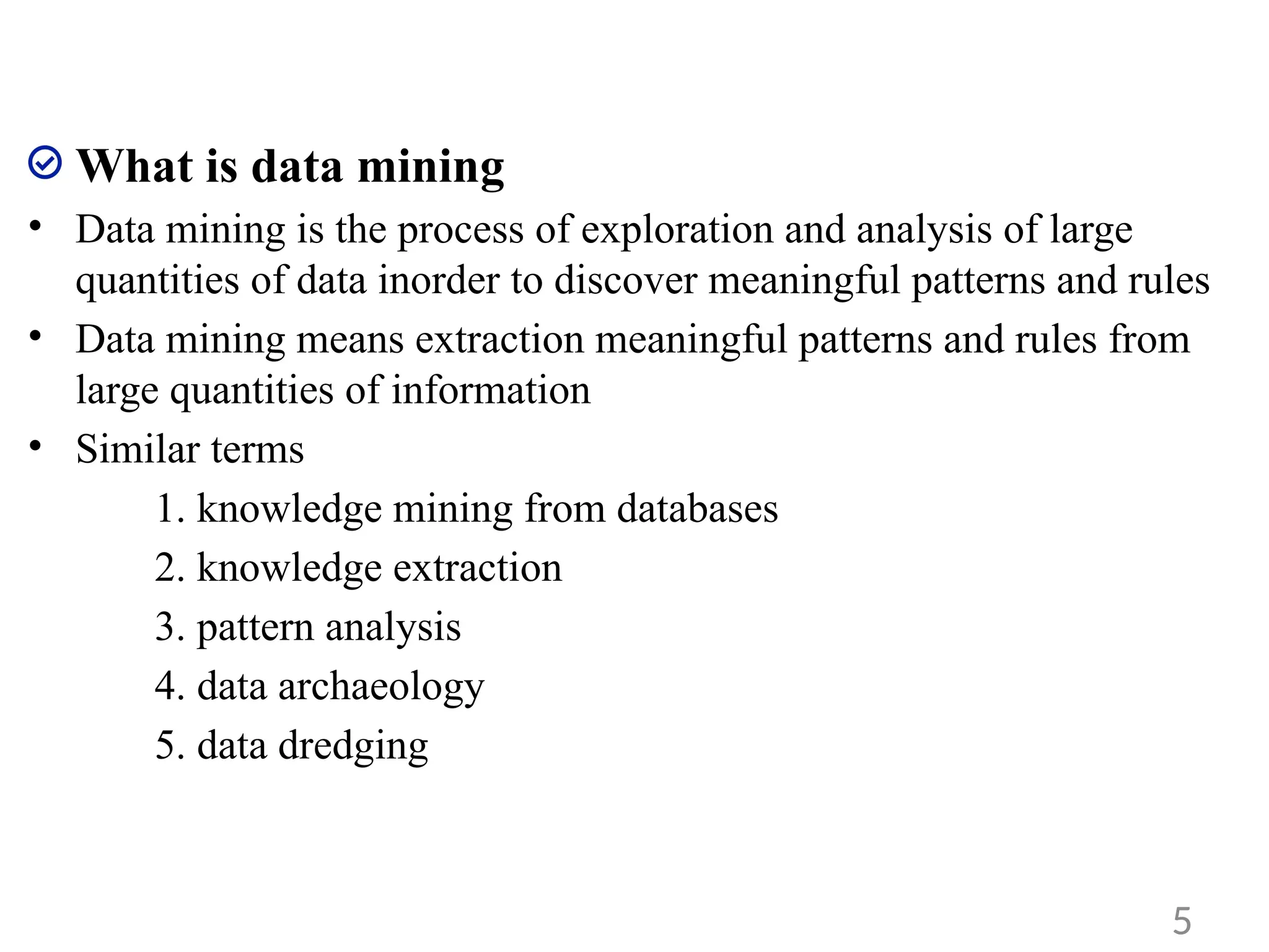
5.
What is datamining
• Data mining is the process of exploration and analysis of large
quantities of data inorder to discover meaningful patterns and rules
• Data mining means extraction meaningful patterns and rules from
large quantities of information
• Similar terms
1. knowledge mining from databases
2. knowledge extraction
3. pattern analysis
4. data archaeology
5. data dredging
5
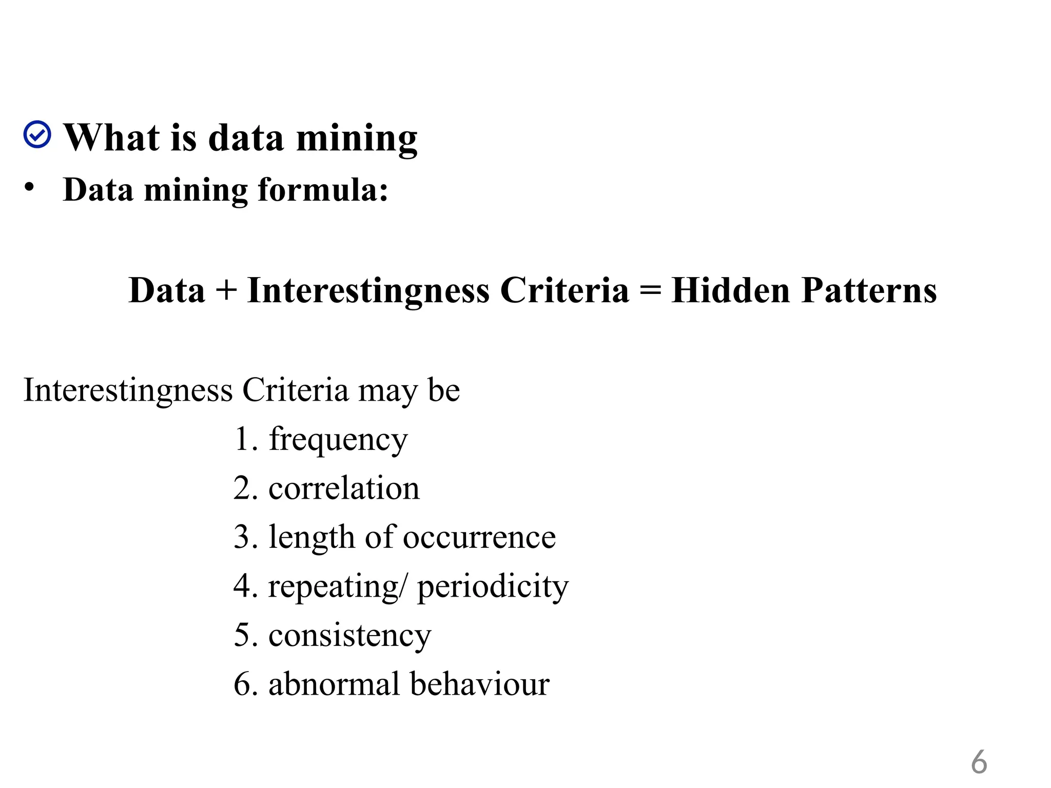
6.
What is datamining
• Data mining formula:
Data + Interestingness Criteria = Hidden Patterns
Interestingness Criteria may be
1. frequency
2. correlation
3. length of occurrence
4. repeating/ periodicity
5. consistency
6. abnormal behaviour
6
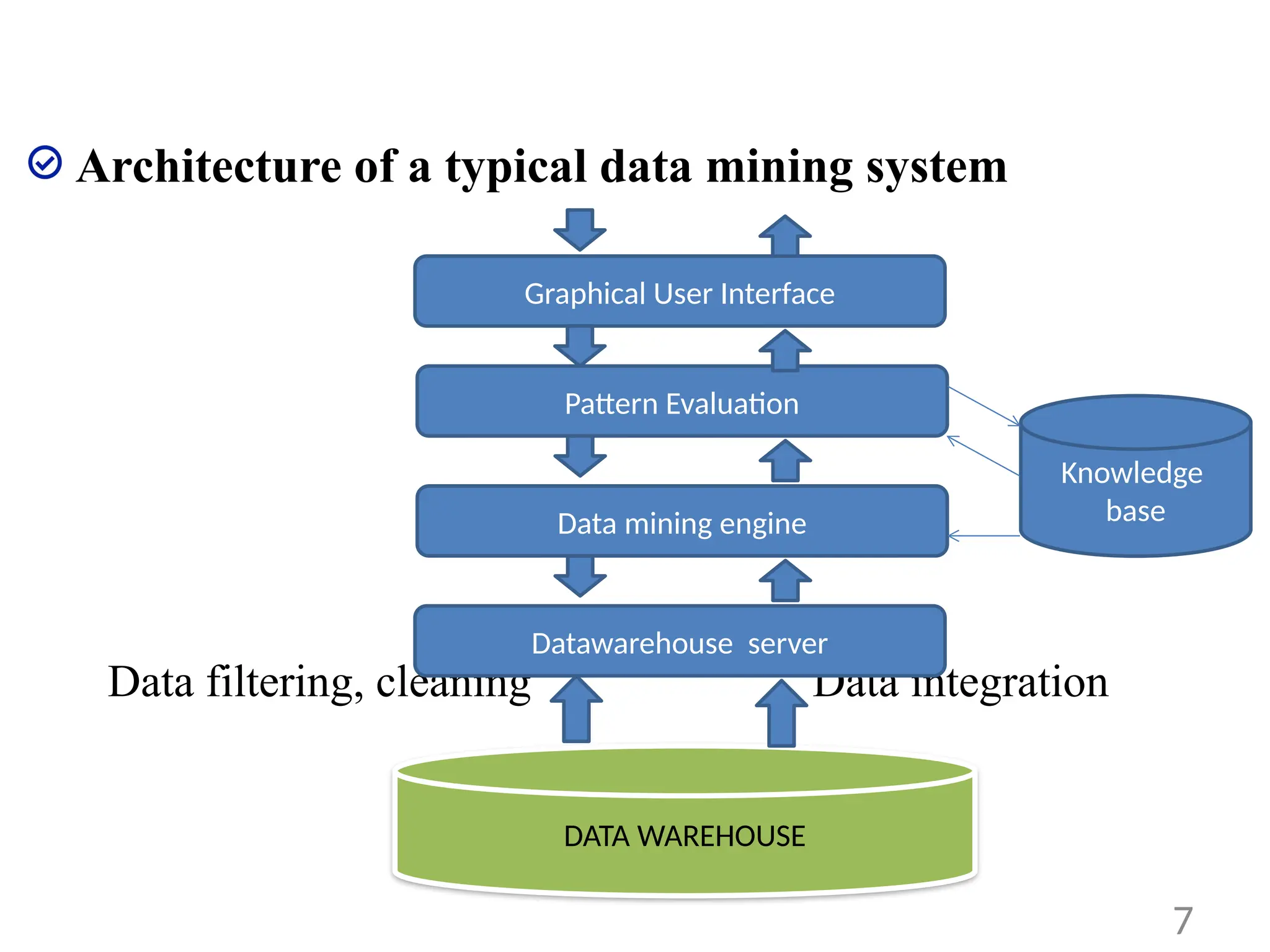
7.
Architecture of atypical data mining system
Data filtering, cleaning Data integration
7
DATA WAREHOUSE
Datawarehouse server
Data mining engine
Pattern Evaluation
Graphical User Interface
Knowledge
base
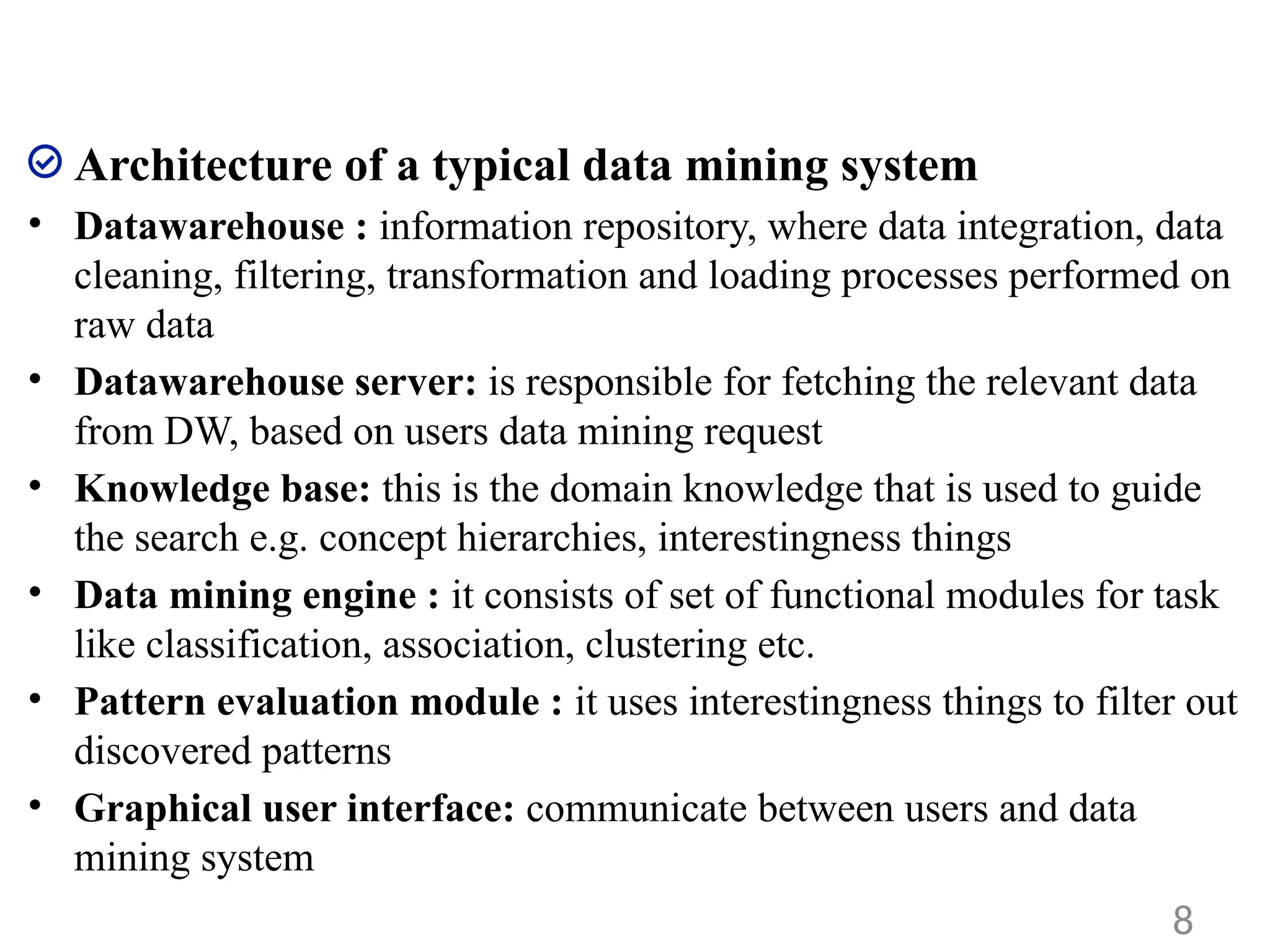
8.
Architecture of atypical data mining system
• Datawarehouse : information repository, where data integration, data
cleaning, filtering, transformation and loading processes performed on
raw data
• Datawarehouse server: is responsible for fetching the relevant data
from DW, based on users data mining request
• Knowledge base: this is the domain knowledge that is used to guide
the search e.g. concept hierarchies, interestingness things
• Data mining engine : it consists of set of functional modules for task
like classification, association, clustering etc.
• Pattern evaluation module : it uses interestingness things to filter out
discovered patterns
• Graphical user interface: communicate between users and data
mining system
8
9.
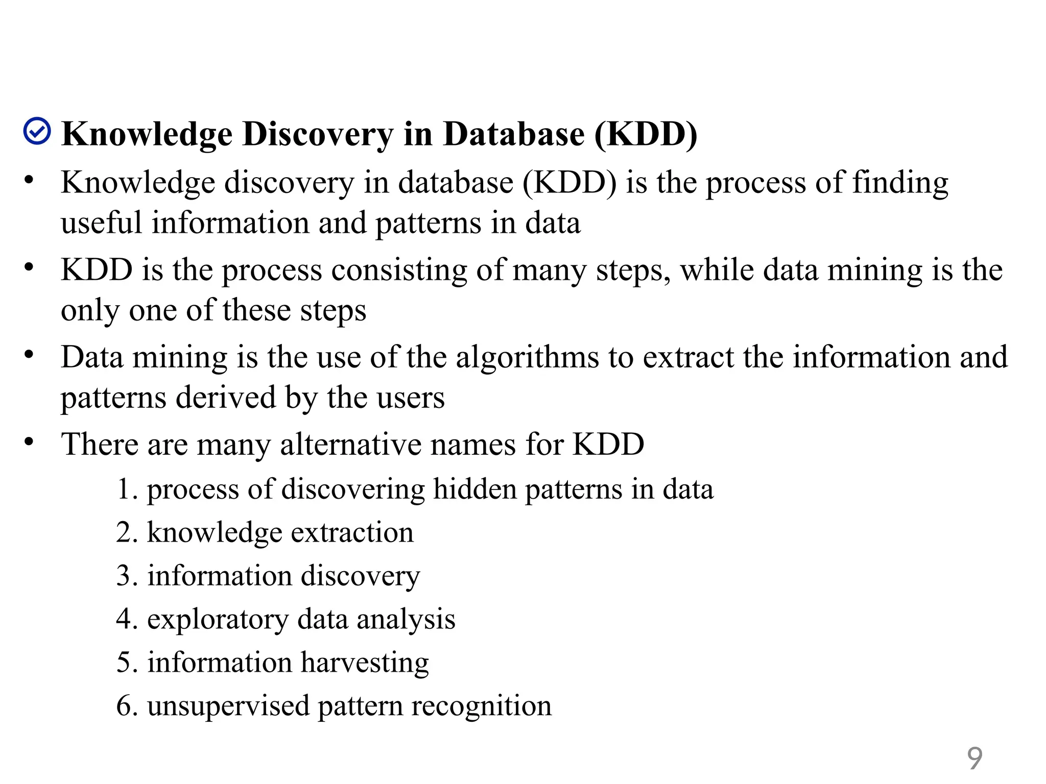
Knowledge Discovery inDatabase (KDD)
• Knowledge discovery in database (KDD) is the process of finding
useful information and patterns in data
• KDD is the process consisting of many steps, while data mining is the
only one of these steps
• Data mining is the use of the algorithms to extract the information and
patterns derived by the users
• There are many alternative names for KDD
1. process of discovering hidden patterns in data
2. knowledge extraction
3. information discovery
4. exploratory data analysis
5. information harvesting
6. unsupervised pattern recognition
9
10.
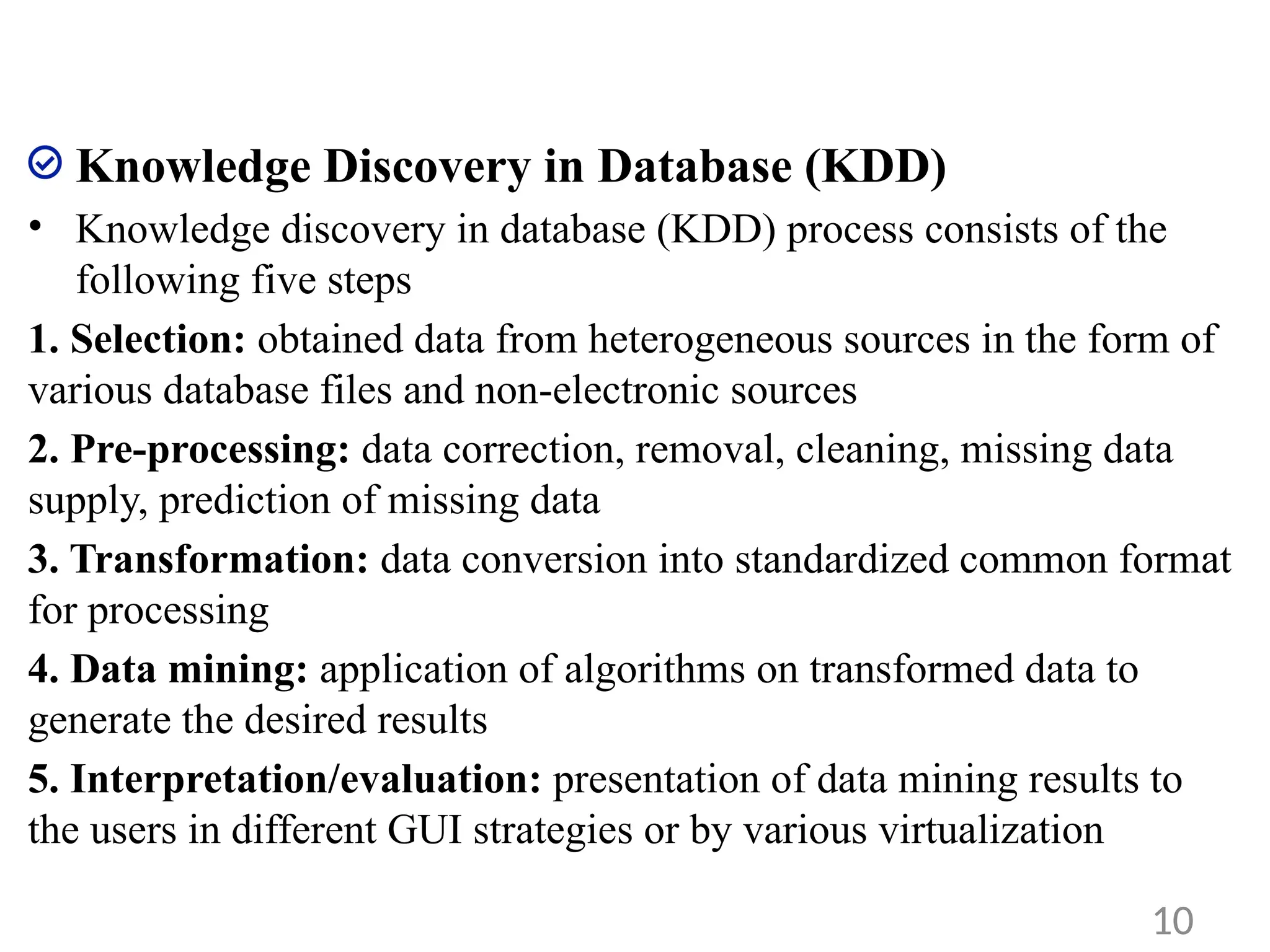
Knowledge Discovery inDatabase (KDD)
• Knowledge discovery in database (KDD) process consists of the
following five steps
1. Selection: obtained data from heterogeneous sources in the form of
various database files and non-electronic sources
2. Pre-processing: data correction, removal, cleaning, missing data
supply, prediction of missing data
3. Transformation: data conversion into standardized common format
for processing
4. Data mining: application of algorithms on transformed data to
generate the desired results
5. Interpretation/evaluation: presentation of data mining results to
the users in different GUI strategies or by various virtualization
10
11.
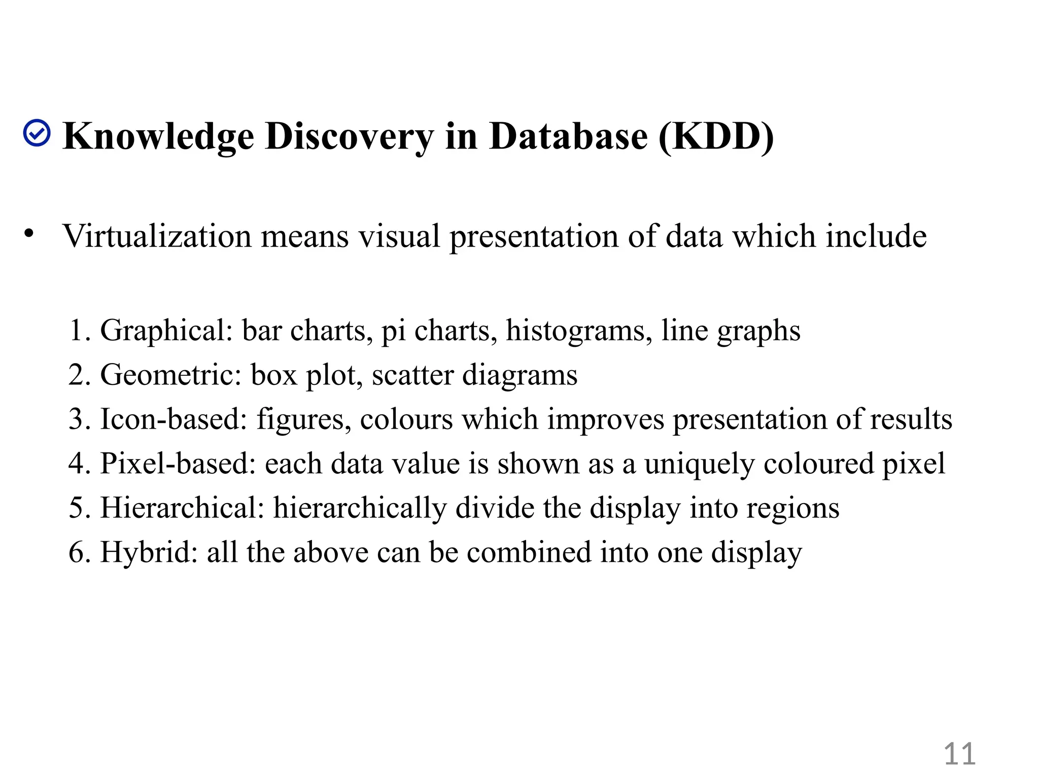
Knowledge Discovery inDatabase (KDD)
• Virtualization means visual presentation of data which include
1. Graphical: bar charts, pi charts, histograms, line graphs
2. Geometric: box plot, scatter diagrams
3. Icon-based: figures, colours which improves presentation of results
4. Pixel-based: each data value is shown as a uniquely coloured pixel
5. Hierarchical: hierarchically divide the display into regions
6. Hybrid: all the above can be combined into one display
11
12.
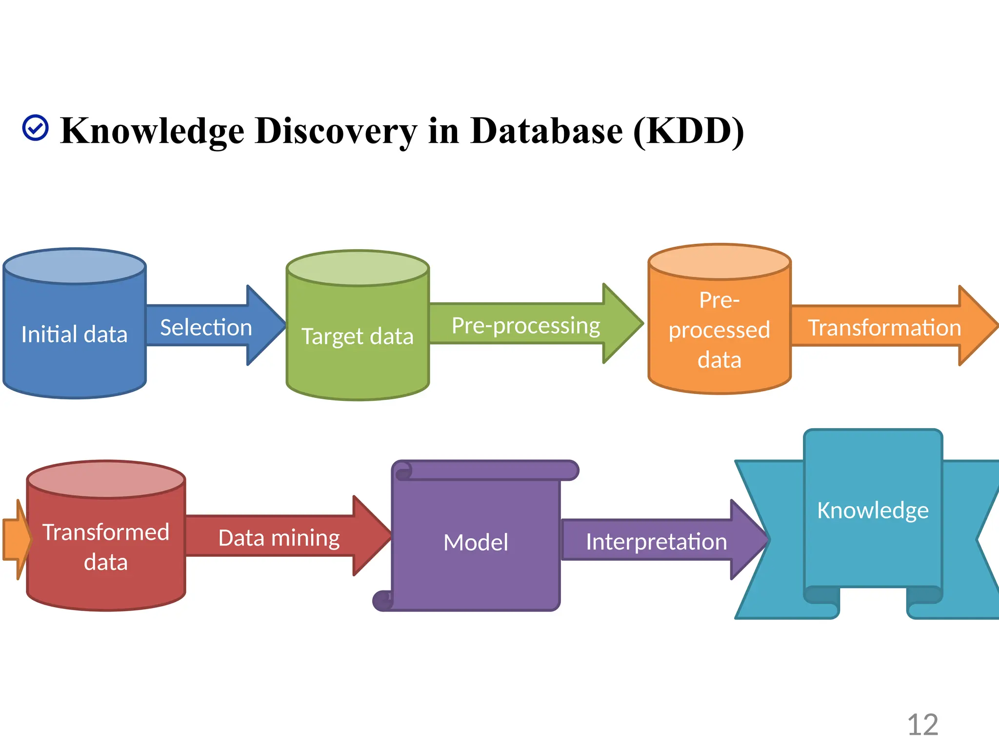
Knowledge Discovery inDatabase (KDD)
• KDD Process
12
Initial data Selection Target data Pre-processing
Pre-
processed
data
Transformation
Transformed
data
Data mining Model Interpretation
Knowledge
13.
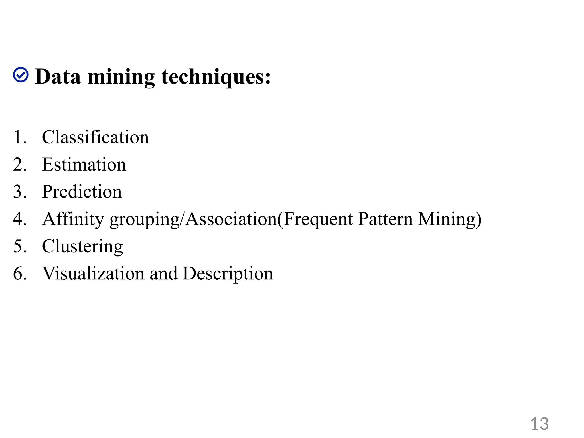
Data mining techniques:
1.Classification
2. Estimation
3. Prediction
4. Affinity grouping/Association(Frequent Pattern Mining)
5. Clustering
6. Visualization and Description
13
14.
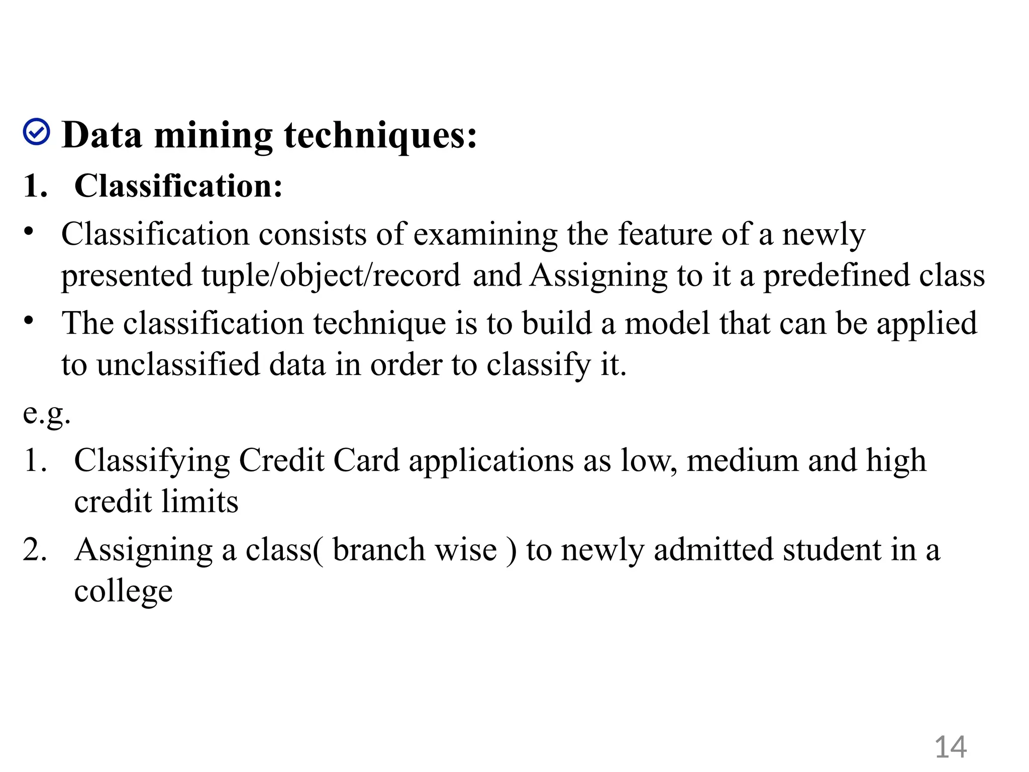
Data mining techniques:
1.Classification:
• Classification consists of examining the feature of a newly
presented tuple/object/record and Assigning to it a predefined class
• The classification technique is to build a model that can be applied
to unclassified data in order to classify it.
e.g.
1. Classifying Credit Card applications as low, medium and high
credit limits
2. Assigning a class( branch wise ) to newly admitted student in a
college
14
15.
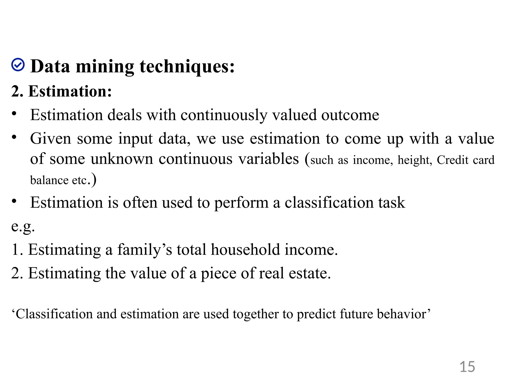
Data mining techniques:
2.Estimation:
• Estimation deals with continuously valued outcome
• Given some input data, we use estimation to come up with a value
of some unknown continuous variables (such as income, height, Credit card
balance etc.)
• Estimation is often used to perform a classification task
e.g.
1. Estimating a family’s total household income.
2. Estimating the value of a piece of real estate.
‘Classification and estimation are used together to predict future behavior’
15
16.
Data mining techniques:
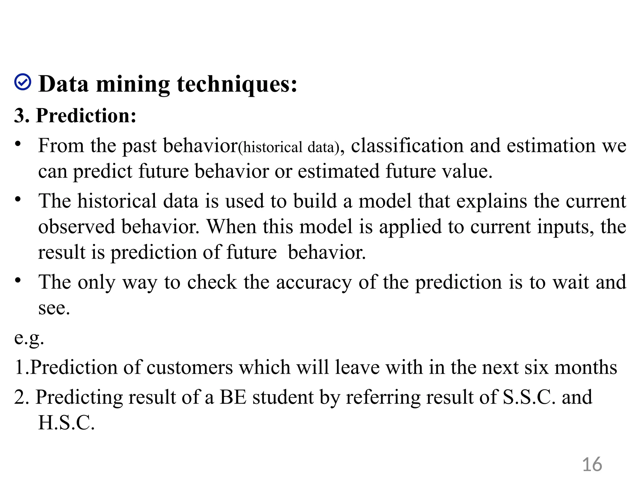
3.Prediction:
• From the past behavior(historical data), classification and estimation we
can predict future behavior or estimated future value.
• The historical data is used to build a model that explains the current
observed behavior. When this model is applied to current inputs, the
result is prediction of future behavior.
• The only way to check the accuracy of the prediction is to wait and
see.
e.g.
1.Prediction of customers which will leave with in the next six months
2. Predicting result of a BE student by referring result of S.S.C. and
H.S.C.
16
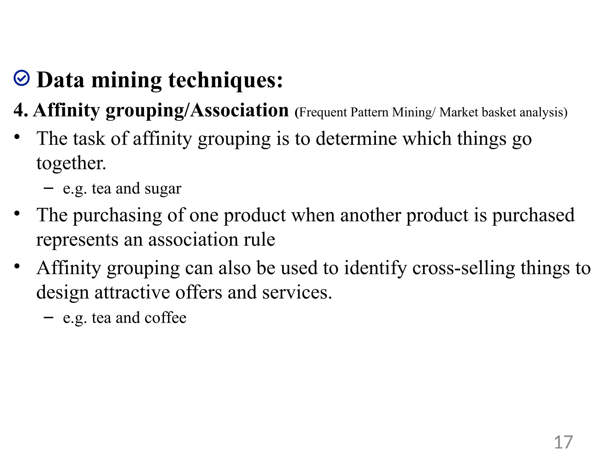
17.
Data mining techniques:
4.Affinity grouping/Association (Frequent Pattern Mining/ Market basket analysis)
• The task of affinity grouping is to determine which things go
together.
– e.g. tea and sugar
• The purchasing of one product when another product is purchased
represents an association rule
• Affinity grouping can also be used to identify cross-selling things to
design attractive offers and services.
– e.g. tea and coffee
17
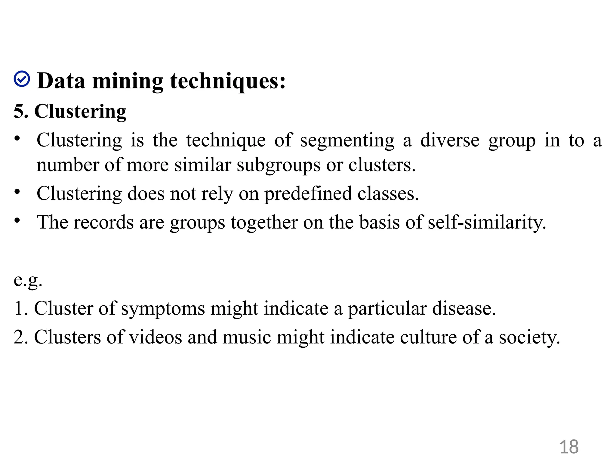
18.
Data mining techniques:
5.Clustering
• Clustering is the technique of segmenting a diverse group in to a
number of more similar subgroups or clusters.
• Clustering does not rely on predefined classes.
• The records are groups together on the basis of self-similarity.
e.g.
1. Cluster of symptoms might indicate a particular disease.
2. Clusters of videos and music might indicate culture of a society.
18
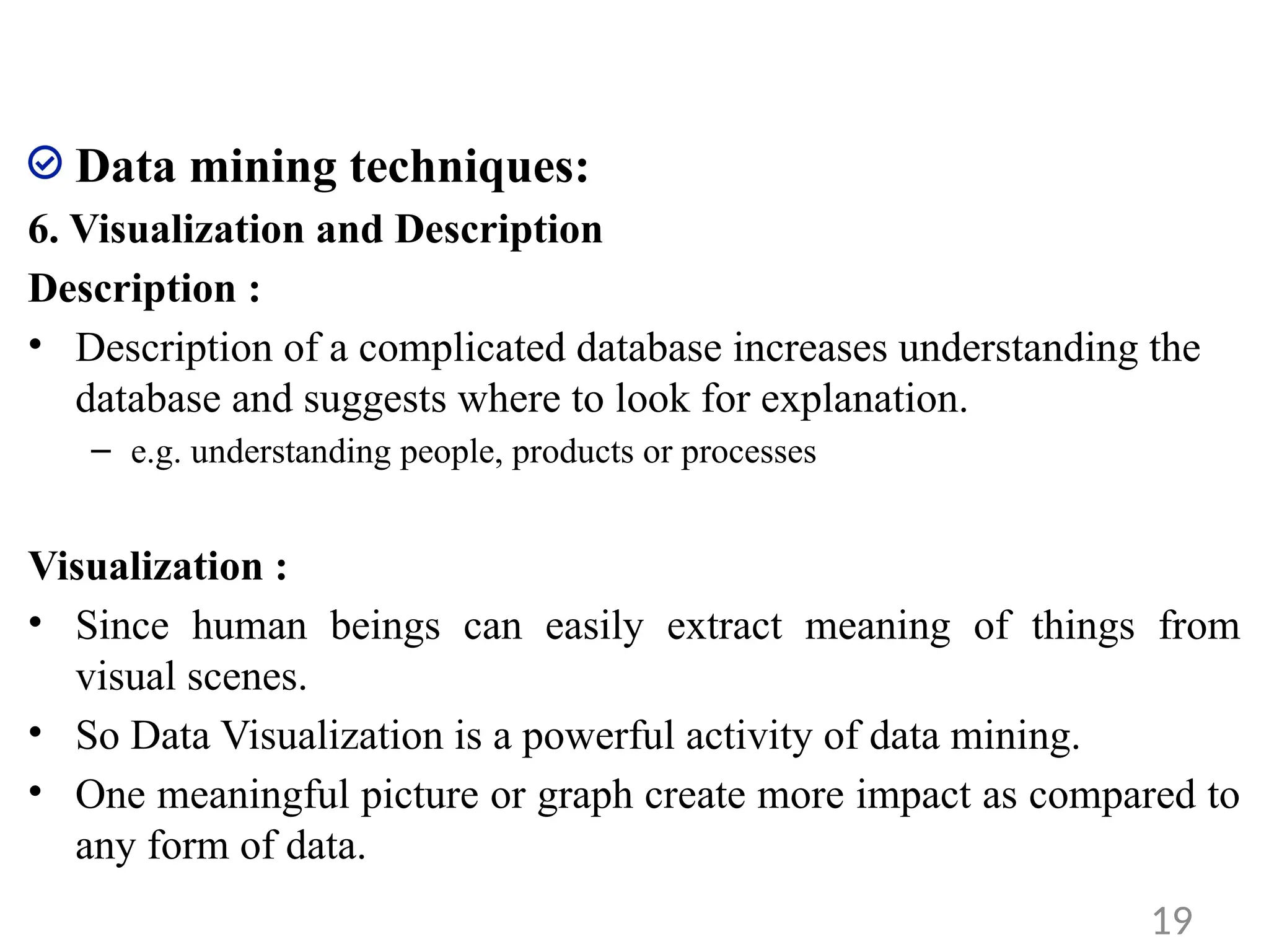
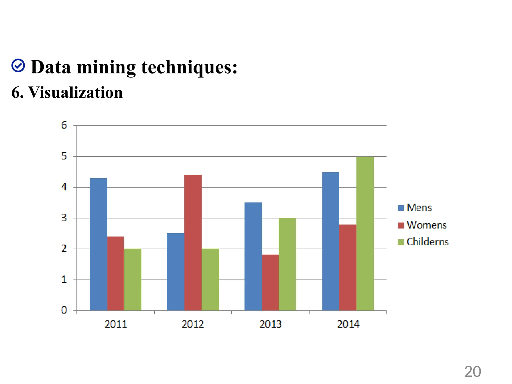
19.
Data mining techniques:
6.Visualization and Description
Description :
• Description of a complicated database increases understanding the
database and suggests where to look for explanation.
– e.g. understanding people, products or processes
Visualization :
• Since human beings can easily extract meaning of things from
visual scenes.
• So Data Visualization is a powerful activity of data mining.
• One meaningful picture or graph create more impact as compared to
any form of data.
19
Data mining algorithms:
differentalgorithms we are going to use for data mining
1. Decision tree
2. Naïve bayes classification (Bayesian)
3. Bootstamp algorithm
4. Random forest
5. K-means clustering
6. Agglomerative algorithm
7. Divisive algorithm
8. BRICH algorithm
9. DBSCAN and OPTICS algorithm
10. Apriori algorithm
11. Market basket analysis
21
22.
Applications of Datamining:
data mining is widely used in divers areas, there are number of
commercial data mining system available
1. Financial data analysis
2. Retail industry
3. Telecommunication industry
4. Biological data analysis
5. Intrusion detection
6. Other scientific applications (geosciences, astronomy, climate and
ecosystem modeling, chemical engineering, fluid dynamics etc)
22
23.
Issues in Datamining:
• Human interaction: domain knowledge experts, technical experts
needed to formulate queries, identify training data set and able to
visualize desired results
• Interpretation of result: required experts to correctly interpret the
result
• Visualization of results: to easily view and understand the o/p of
data mining algorithms, Visualization of the results is helpful
• Large datasets: massive datasets create problems with different
modeling applications
• High dimensionality: use of so many attributes may increase
overall complexity and decreases the efficiency
23
24.
Issues in Datamining:
• Multimedia data: the use of multimedia data complicates or
invalidates many proposed algorithms
• Missing data: missing data can lead to invalid results(incorrect)
• Irrelevant data: some attributes might not be of interest to data
mining or may not be useful
• Noisy data: attribute values might be incorrect or invalid
• Changing data: databases can not be assumed to be static e.g.
address, marital status or age
24
Data Exploration Definition:
Data exploration is an approach similar to initial data analysis,
whereby a data analyst uses visual exploration to understand what is
in a dataset and the characteristics of the data, rather than through
traditional data management systems.
26
27.
Attributes
• An attributeis a data field, representing a characteristic or feature
of a data object.
• The nouns attribute, dimension, feature, and variable are often used
interchangeably in the literature.
• The term dimension is commonly used in data warehousing.
• Machine learning literature tends to use the term feature, while
statisticians prefer the term variable.
• Data mining and database professionals commonly use the term
attribute
• Attributes describing a customer object can include: customer ID,
name, and address.
27
28.
Types of Attributes
1.Nominal attributes
2. Binary attributes
3. Ordinal attributes
4. Numeric attributes
a) Interval-scaled attributes
b) Ratio-scaled attributes
28
29.
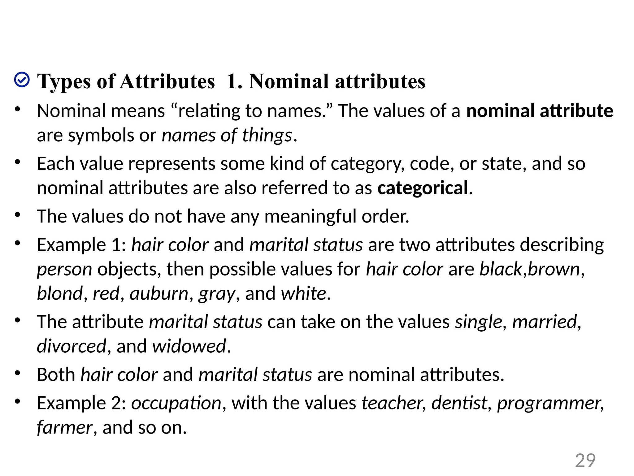
Types of Attributes1. Nominal attributes
• Nominal means “relating to names.” The values of a nominal attribute
are symbols or names of things.
• Each value represents some kind of category, code, or state, and so
nominal attributes are also referred to as categorical.
• The values do not have any meaningful order.
• Example 1: hair color and marital status are two attributes describing
person objects, then possible values for hair color are black,brown,
blond, red, auburn, gray, and white.
• The attribute marital status can take on the values single, married,
divorced, and widowed.
• Both hair color and marital status are nominal attributes.
• Example 2: occupation, with the values teacher, dentist, programmer,
farmer, and so on.
29
30.
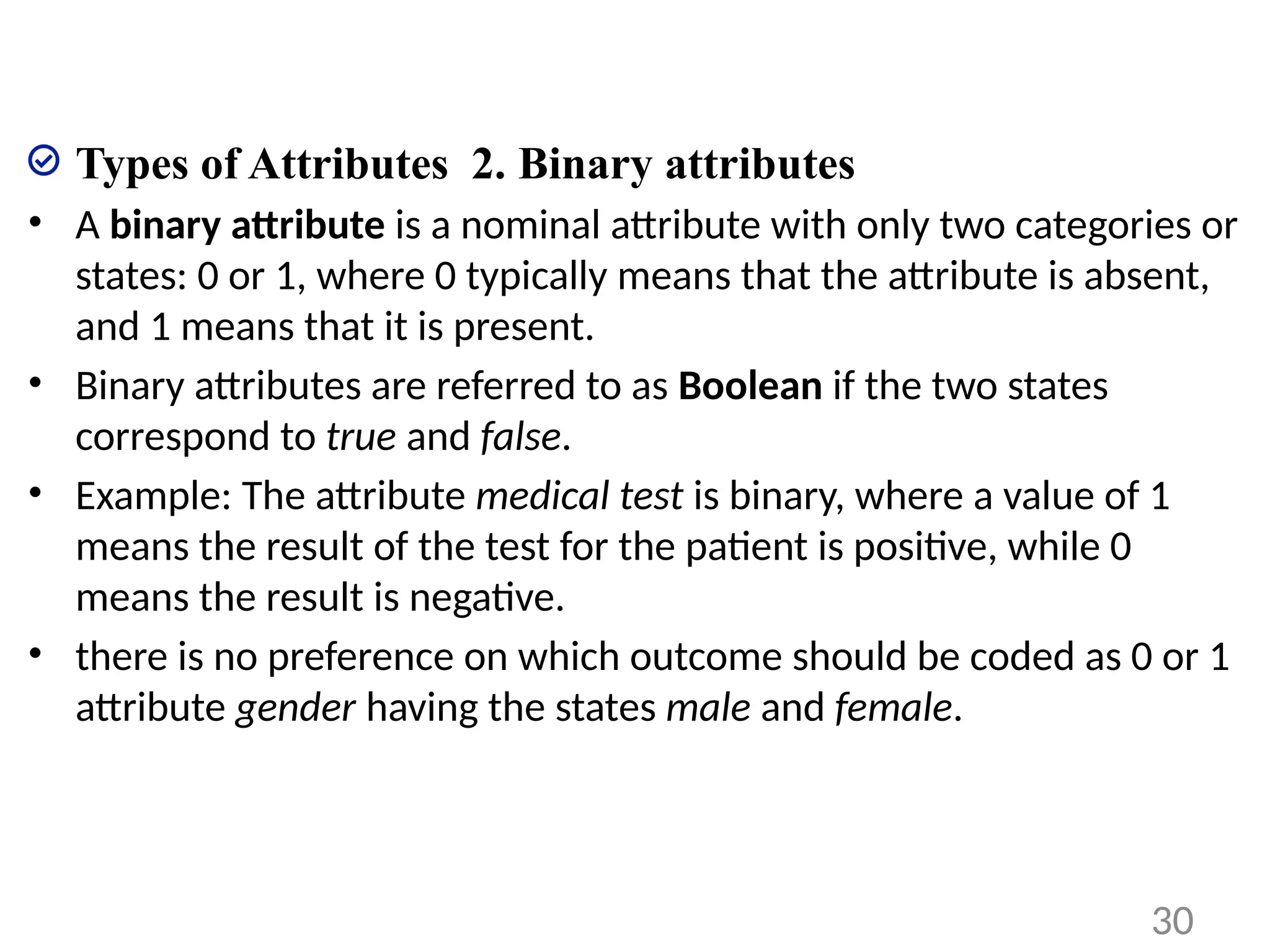
Types of Attributes2. Binary attributes
• A binary attribute is a nominal attribute with only two categories or
states: 0 or 1, where 0 typically means that the attribute is absent,
and 1 means that it is present.
• Binary attributes are referred to as Boolean if the two states
correspond to true and false.
• Example: The attribute medical test is binary, where a value of 1
means the result of the test for the patient is positive, while 0
means the result is negative.
• there is no preference on which outcome should be coded as 0 or 1
attribute gender having the states male and female.
30
31.
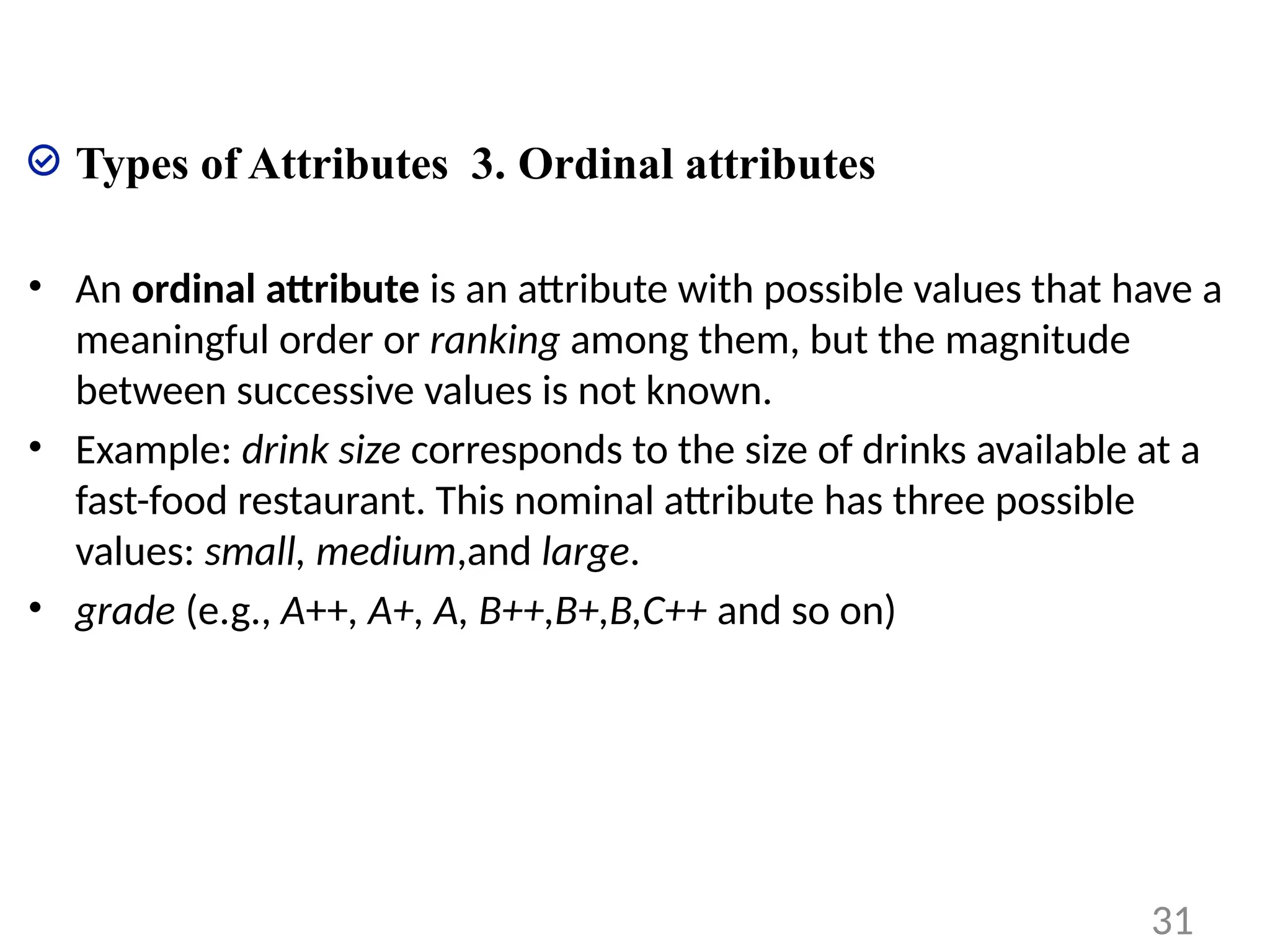
Types of Attributes3. Ordinal attributes
• An ordinal attribute is an attribute with possible values that have a
meaningful order or ranking among them, but the magnitude
between successive values is not known.
• Example: drink size corresponds to the size of drinks available at a
fast-food restaurant. This nominal attribute has three possible
values: small, medium,and large.
• grade (e.g., A++, A+, A, B++,B+,B,C++ and so on)
31
32.
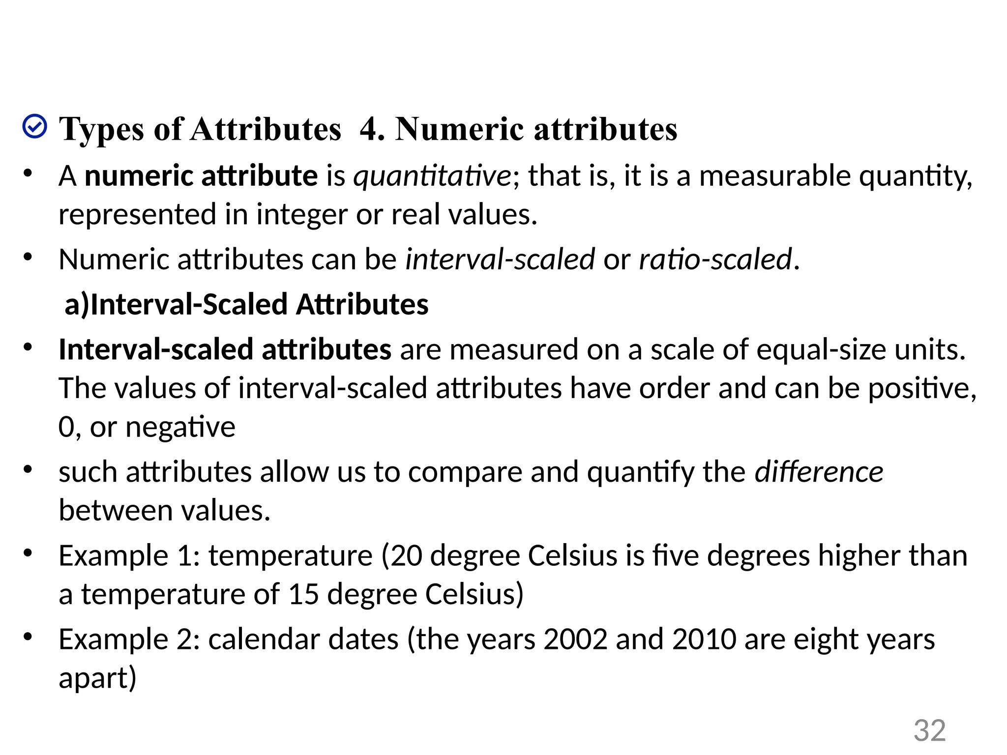
Types of Attributes4. Numeric attributes
• A numeric attribute is quantitative; that is, it is a measurable quantity,
represented in integer or real values.
• Numeric attributes can be interval-scaled or ratio-scaled.
a)Interval-Scaled Attributes
• Interval-scaled attributes are measured on a scale of equal-size units.
The values of interval-scaled attributes have order and can be positive,
0, or negative
• such attributes allow us to compare and quantify the difference
between values.
• Example 1: temperature (20 degree Celsius is five degrees higher than
a temperature of 15 degree Celsius)
• Example 2: calendar dates (the years 2002 and 2010 are eight years
apart)
32
33.
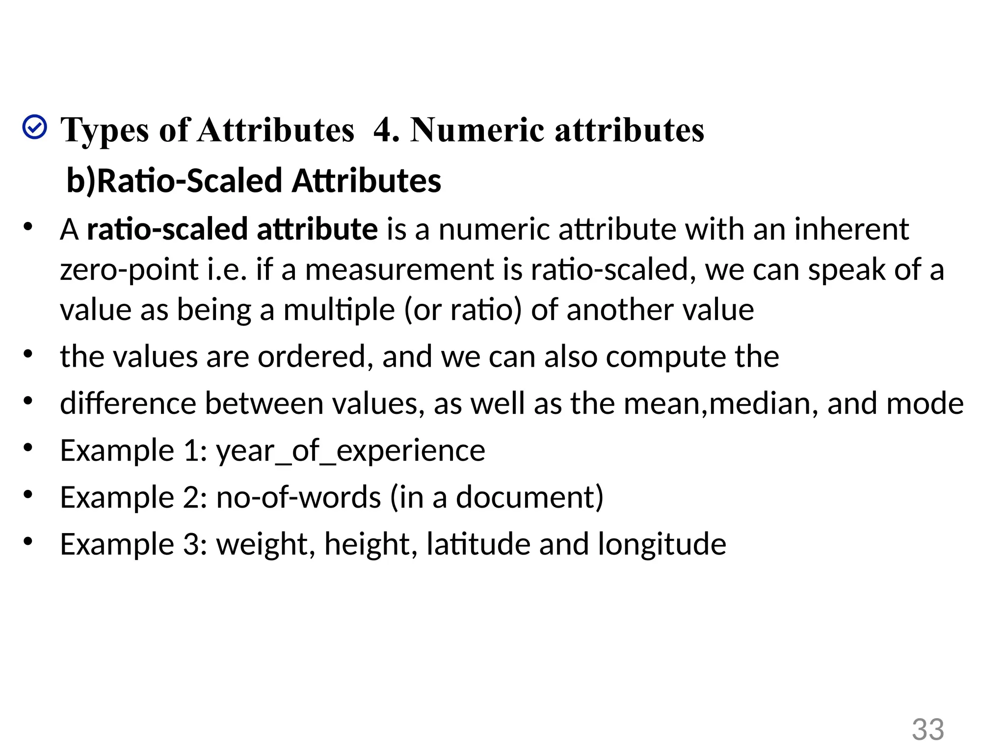
Types of Attributes4. Numeric attributes
b)Ratio-Scaled Attributes
• A ratio-scaled attribute is a numeric attribute with an inherent
zero-point i.e. if a measurement is ratio-scaled, we can speak of a
value as being a multiple (or ratio) of another value
• the values are ordered, and we can also compute the
• difference between values, as well as the mean,median, and mode
• Example 1: year_of_experience
• Example 2: no-of-words (in a document)
• Example 3: weight, height, latitude and longitude
33
34.
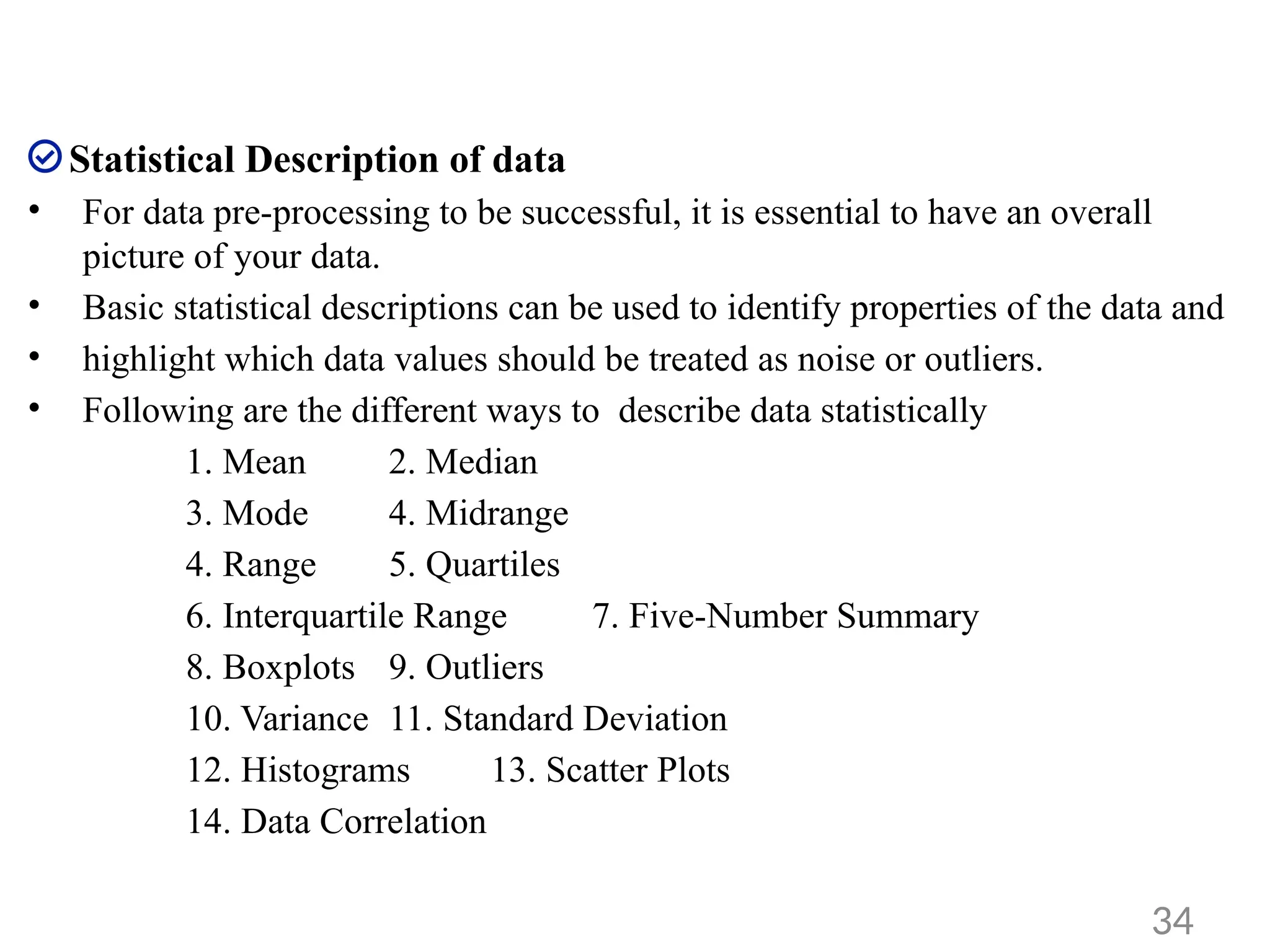
Statistical Description ofdata
• For data pre-processing to be successful, it is essential to have an overall
picture of your data.
• Basic statistical descriptions can be used to identify properties of the data and
• highlight which data values should be treated as noise or outliers.
• Following are the different ways to describe data statistically
1. Mean 2. Median
3. Mode 4. Midrange
4. Range 5. Quartiles
6. Interquartile Range 7. Five-Number Summary
8. Boxplots 9. Outliers
10. Variance 11. Standard Deviation
12. Histograms 13. Scatter Plots
14. Data Correlation
34
35.
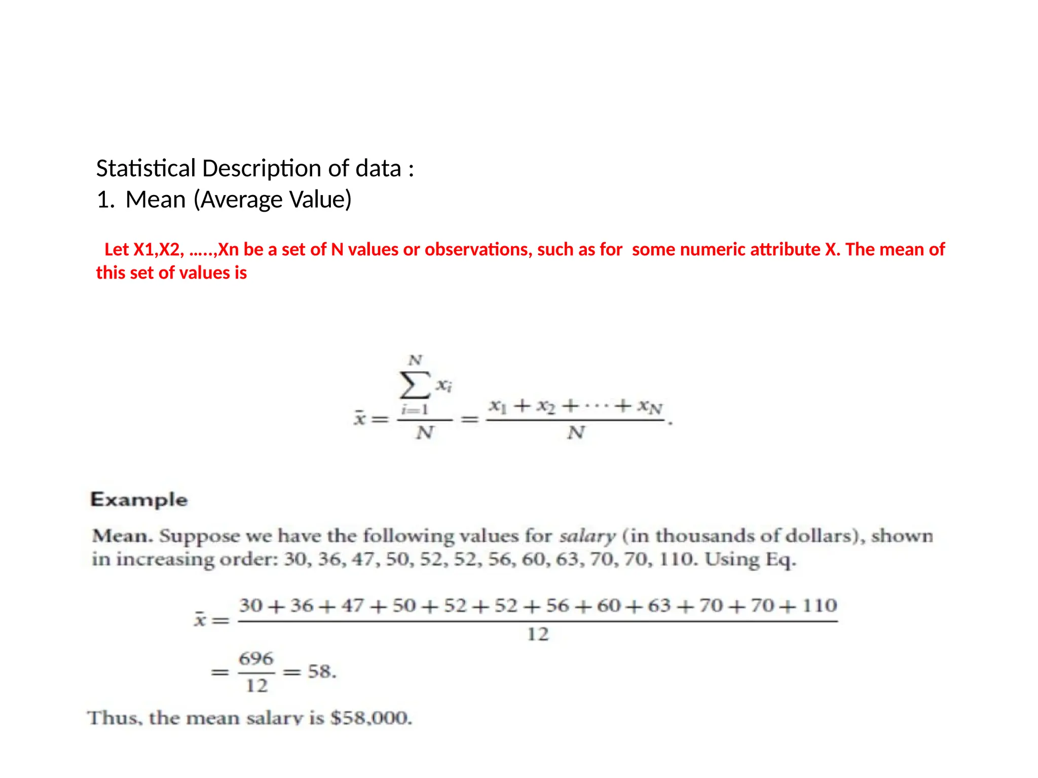
Statistical Description ofdata :
1. Mean (Average Value)
Let X1,X2, …..,Xn be a set of N values or observations, such as for some numeric attribute X. The mean of
this set of values is
36.
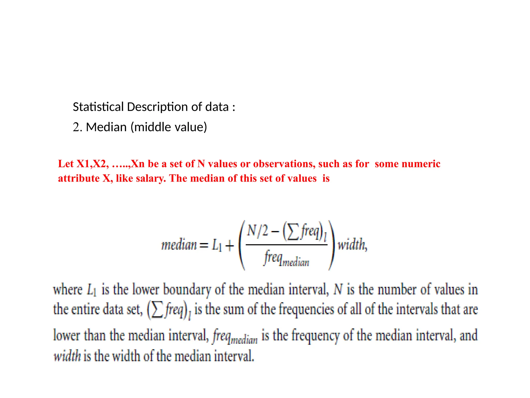
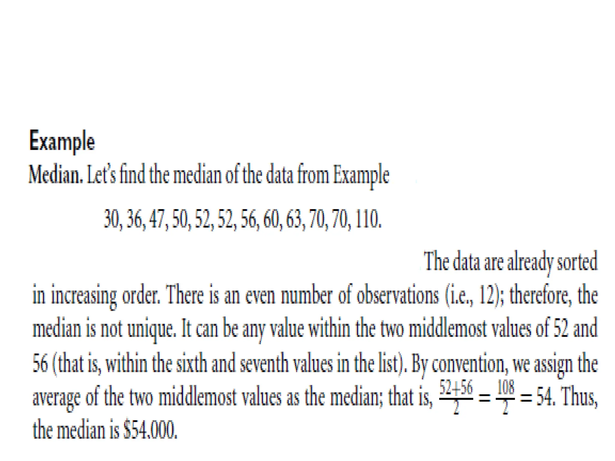
Statistical Description ofdata :
2. Median (middle value)
Let X1,X2, …..,Xn be a set of N values or observations, such as for some numeric
attribute X, like salary. The median of this set of values is
38.
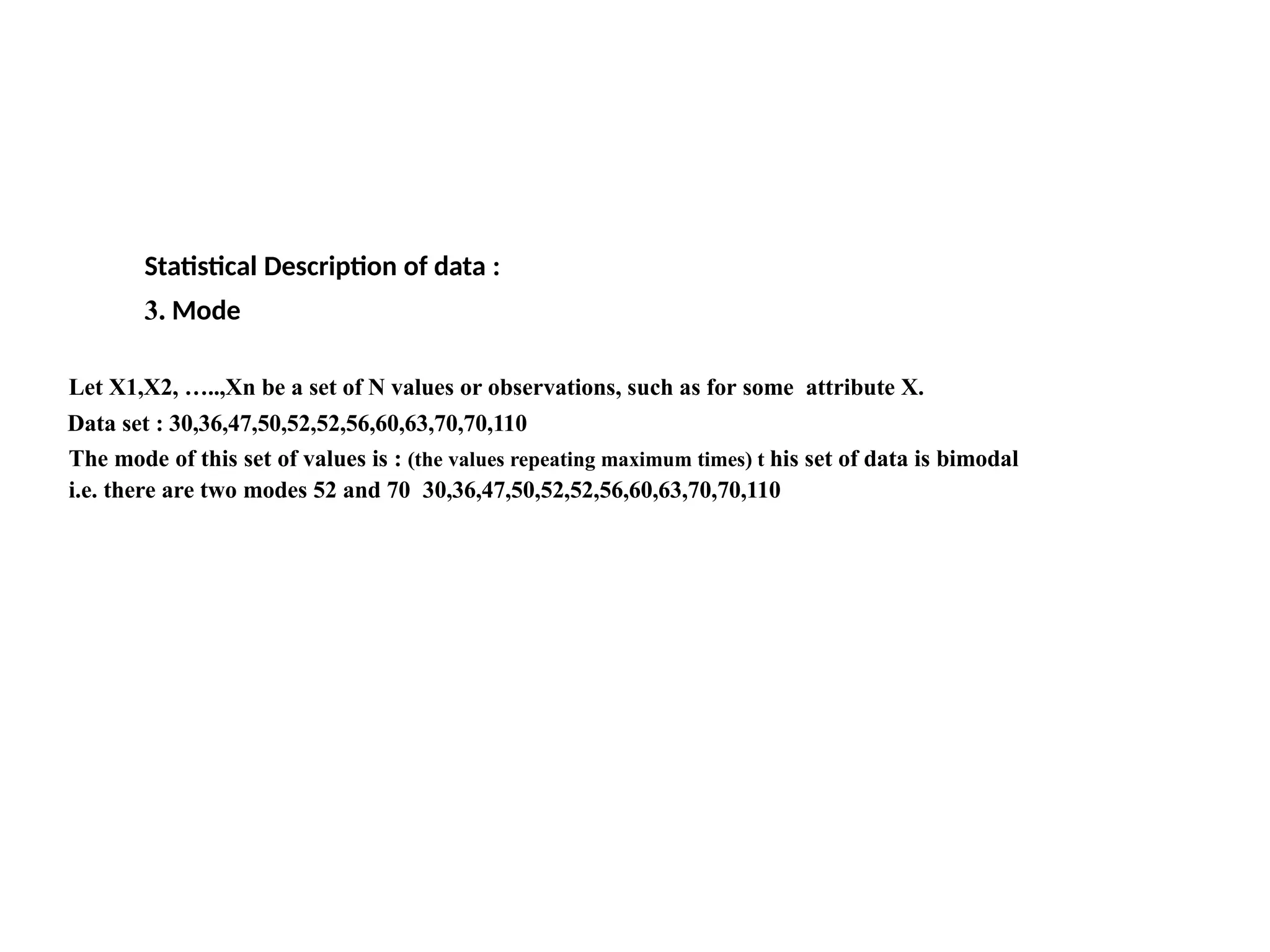
Let X1,X2, …..,Xnbe a set of N values or observations, such as for some attribute X.
Data set : 30,36,47,50,52,52,56,60,63,70,70,110
The mode of this set of values is : (the values repeating maximum times) t his set of data is bimodal
i.e. there are two modes 52 and 70 30,36,47,50,52,52,56,60,63,70,70,110)
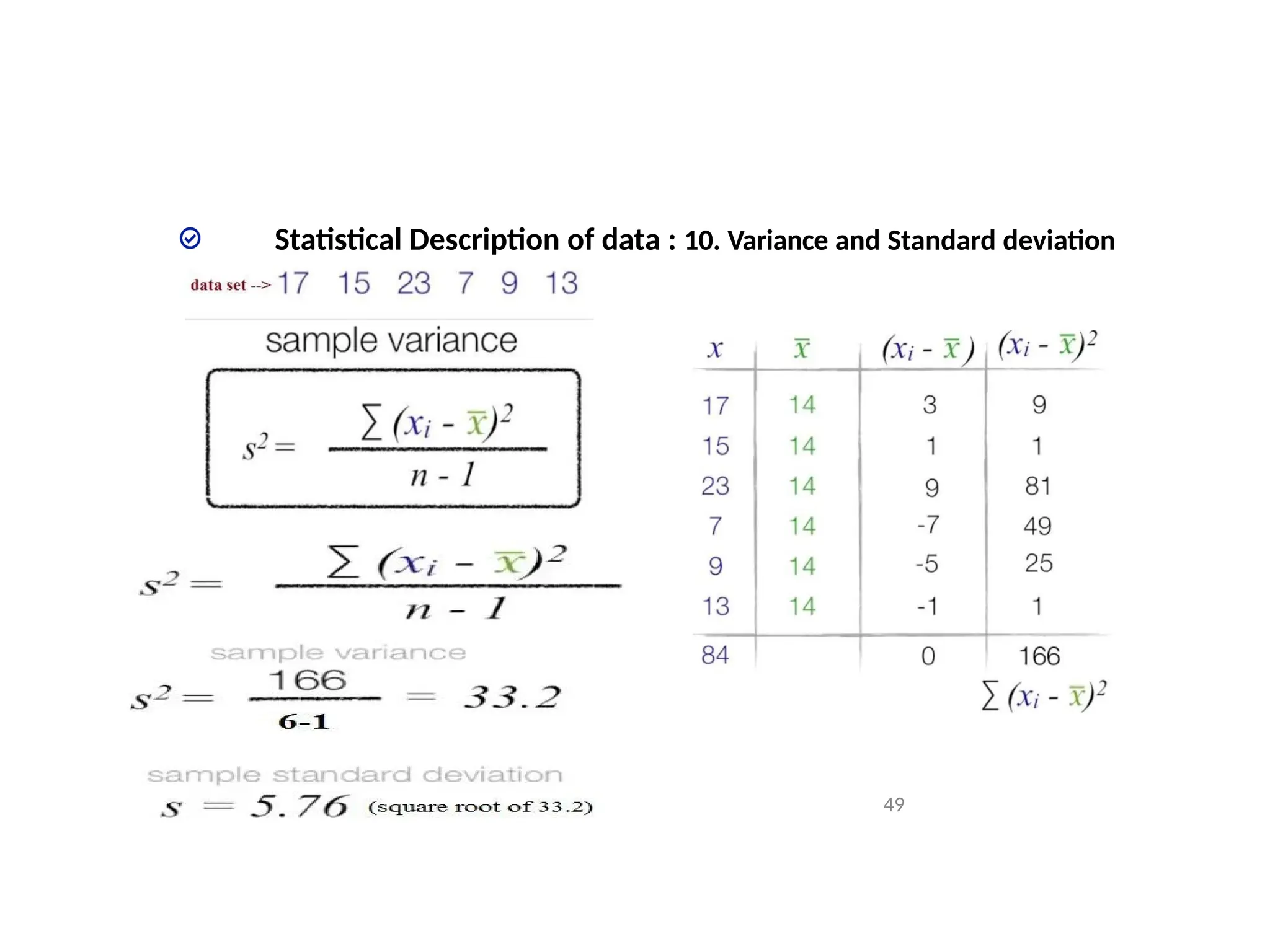
Statistical Description of data :
3. Mode
39.
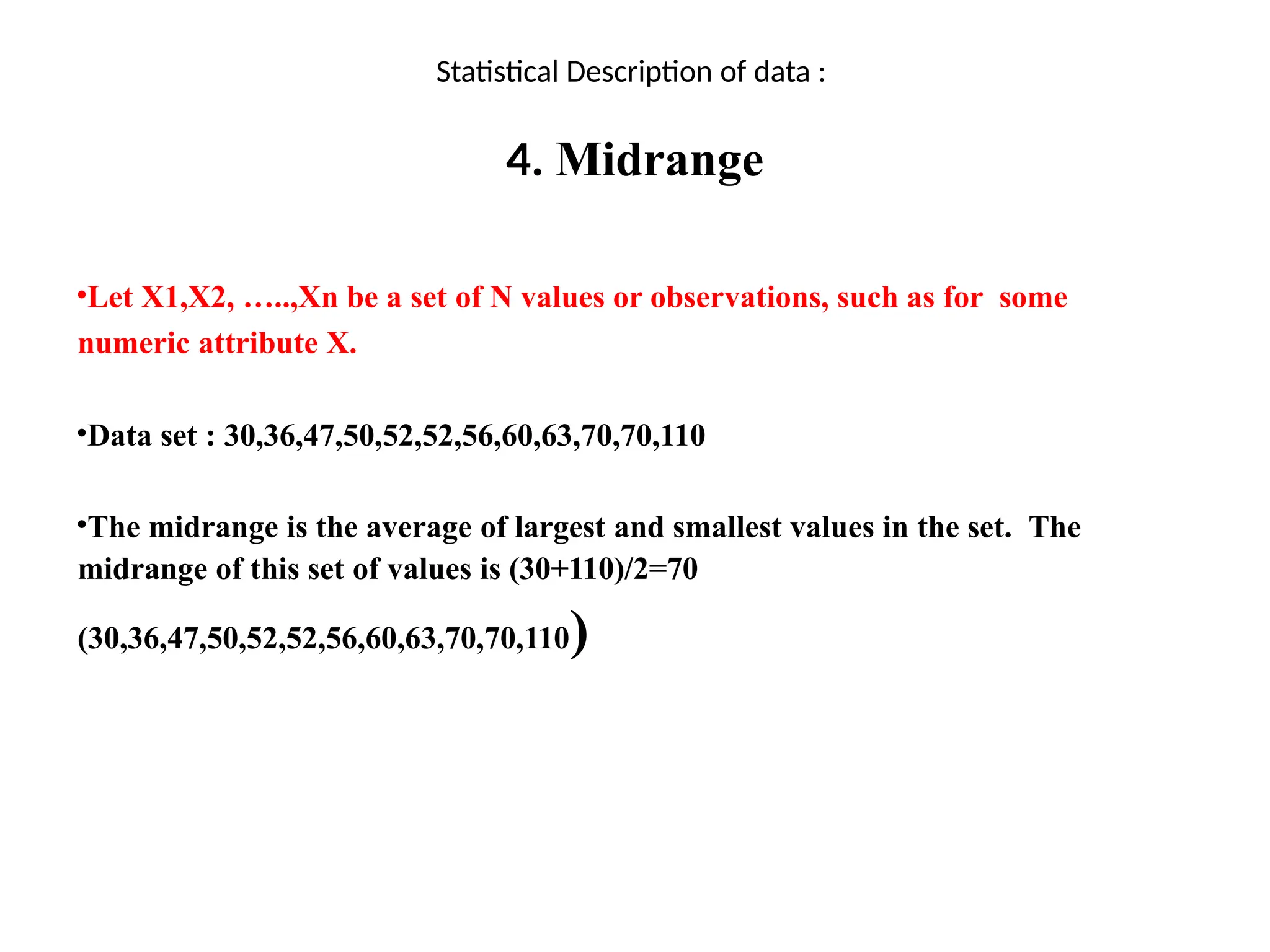
Statistical Description ofdata :
4. Midrange
•Let X1,X2, …..,Xn be a set of N values or observations, such as for some
numeric attribute X.
•Data set : 30,36,47,50,52,52,56,60,63,70,70,110
•The midrange is the average of largest and smallest values in the set. The
midrange of this set of values is (30+110)/2=70
(30,36,47,50,52,52,56,60,63,70,70,110)
40.
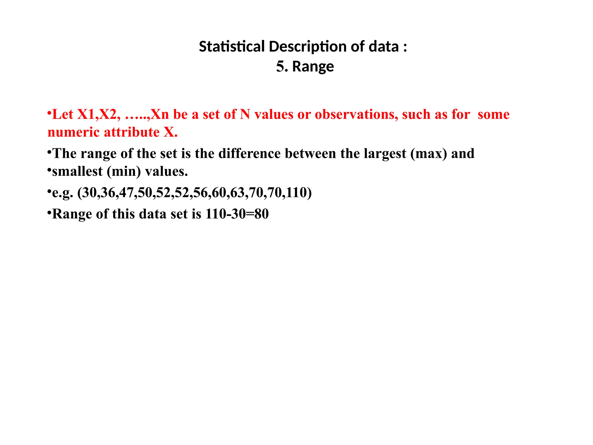
Statistical Description ofdata :
5. Range
•Let X1,X2, …..,Xn be a set of N values or observations, such as for some
numeric attribute X.
•The range of the set is the difference between the largest (max) and
•smallest (min) values.
•e.g. (30,36,47,50,52,52,56,60,63,70,70,110)
•Range of this data set is 110-30=80
41.
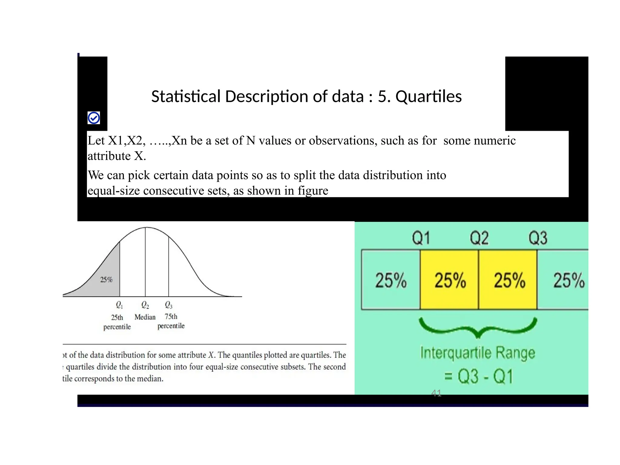
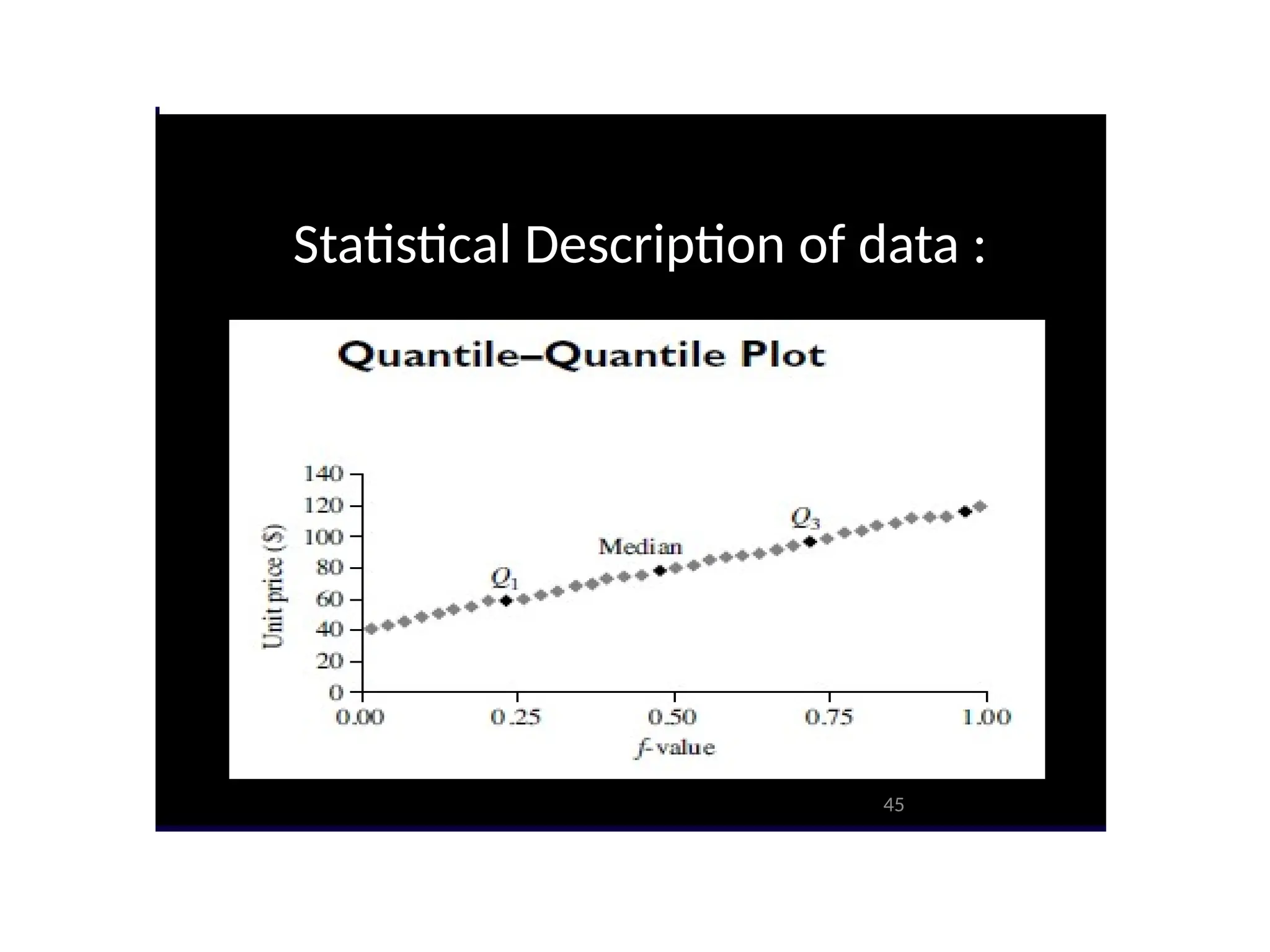
Statistical Description ofdata : 5. Quartiles
Let X1,X2, …..,Xn be a set of N values or observations, such as for some numeric
attribute X.
We can pick certain data points so as to split the data distribution into
equal-size consecutive sets, as shown in figure
41
42.
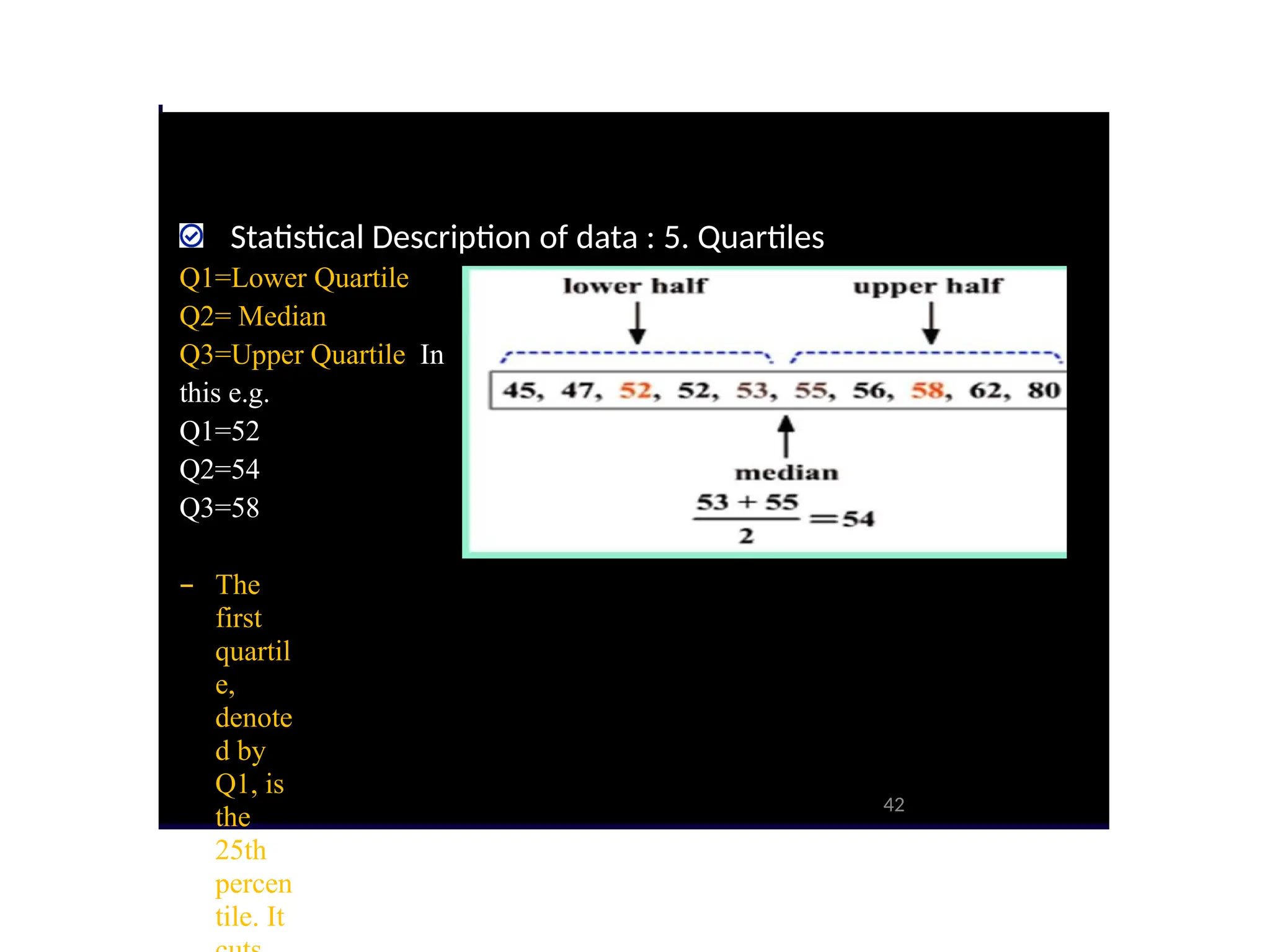
Statistical Description ofdata : 5. Quartiles
Q1=Lower Quartile
Q2= Median
Q3=Upper Quartile In
this e.g.
Q1=52
Q2=54
Q3=58
– The
first
quartil
e,
denote
d by
Q1, is
the
25th
percen
tile. It
42
43.
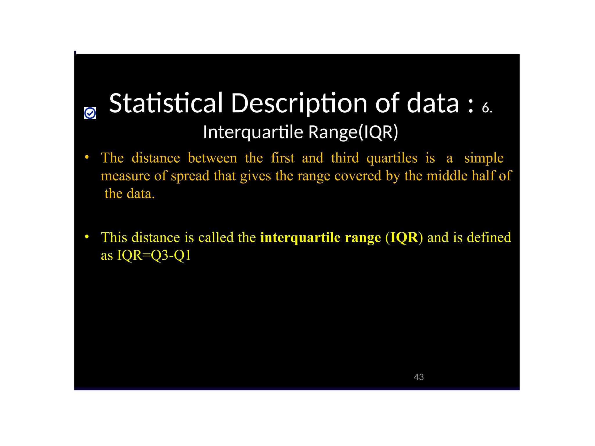
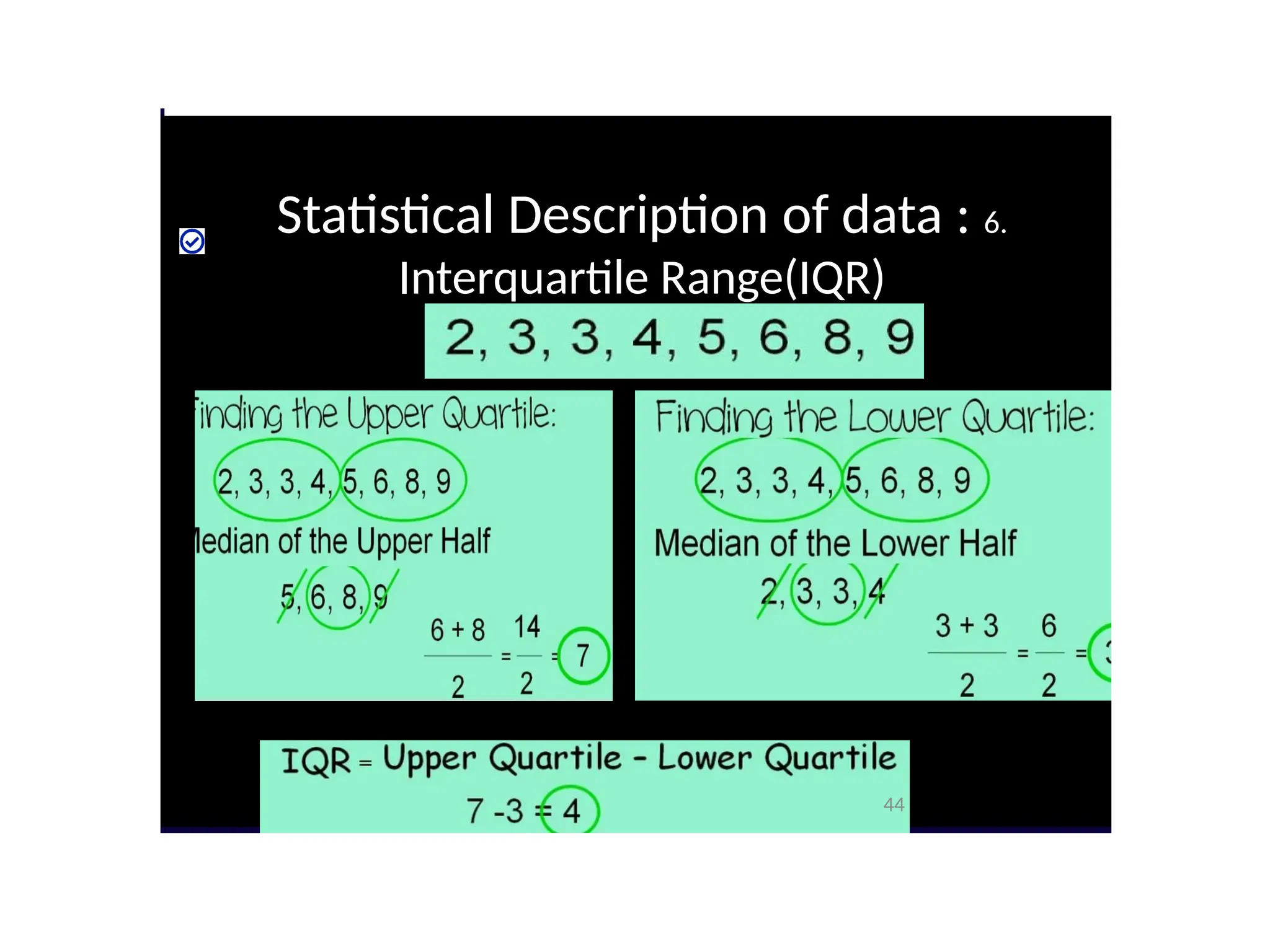
Statistical Description ofdata : 6.
Interquartile Range(IQR)
43
• The distance between the first and third quartiles is a simple
measure of spread that gives the range covered by the middle half of
the data.
• This distance is called the interquartile range (IQR) and is defined
as IQR=Q3-Q1
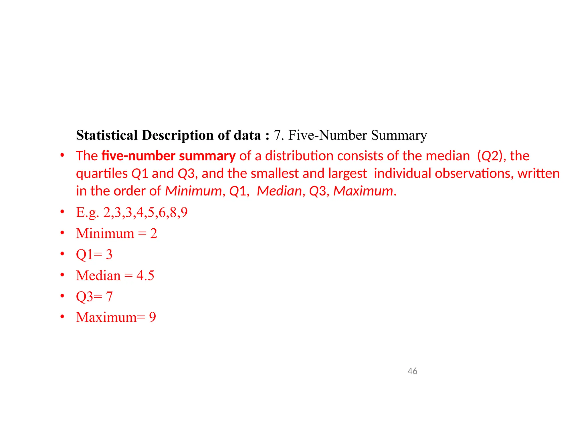
Statistical Description ofdata : 7. Five-Number Summary
• The five-number summary of a distribution consists of the median (Q2), the
quartiles Q1 and Q3, and the smallest and largest individual observations, written
in the order of Minimum, Q1, Median, Q3, Maximum.
• E.g. 2,3,3,4,5,6,8,9
• Minimum = 2
• Q1= 3
• Median = 4.5
• Q3= 7
• Maximum= 9
46
47.
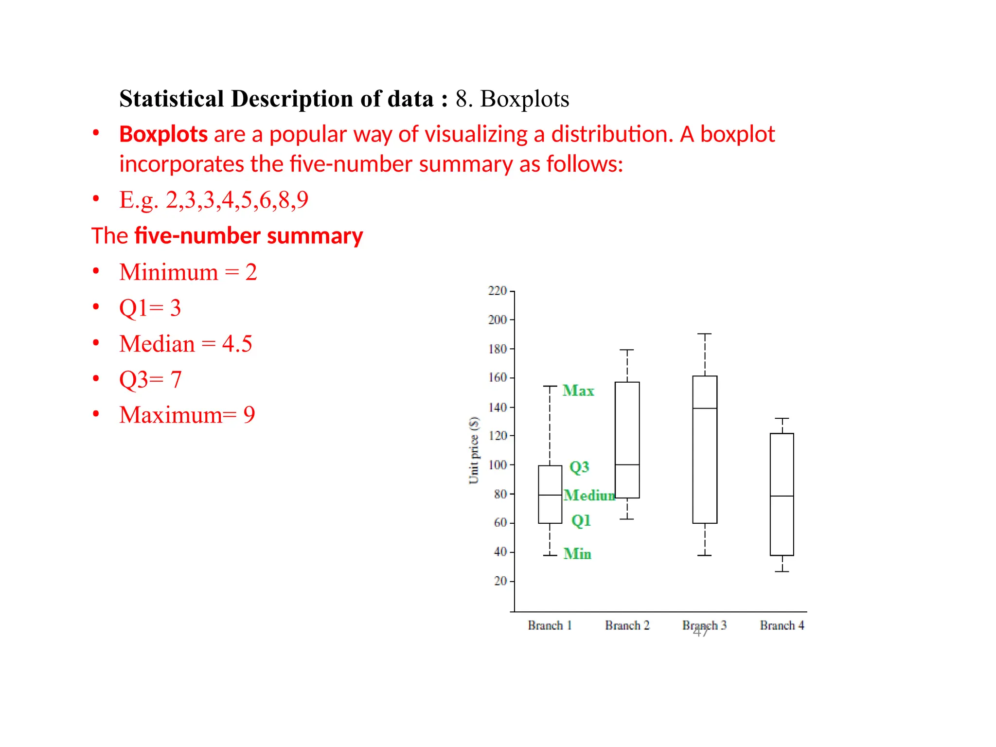
Statistical Description ofdata : 8. Boxplots
• Boxplots are a popular way of visualizing a distribution. A boxplot
incorporates the five-number summary as follows:
• E.g. 2,3,3,4,5,6,8,9
The five-number summary
• Minimum = 2
• Q1= 3
• Median = 4.5
• Q3= 7
• Maximum= 9
47
48.
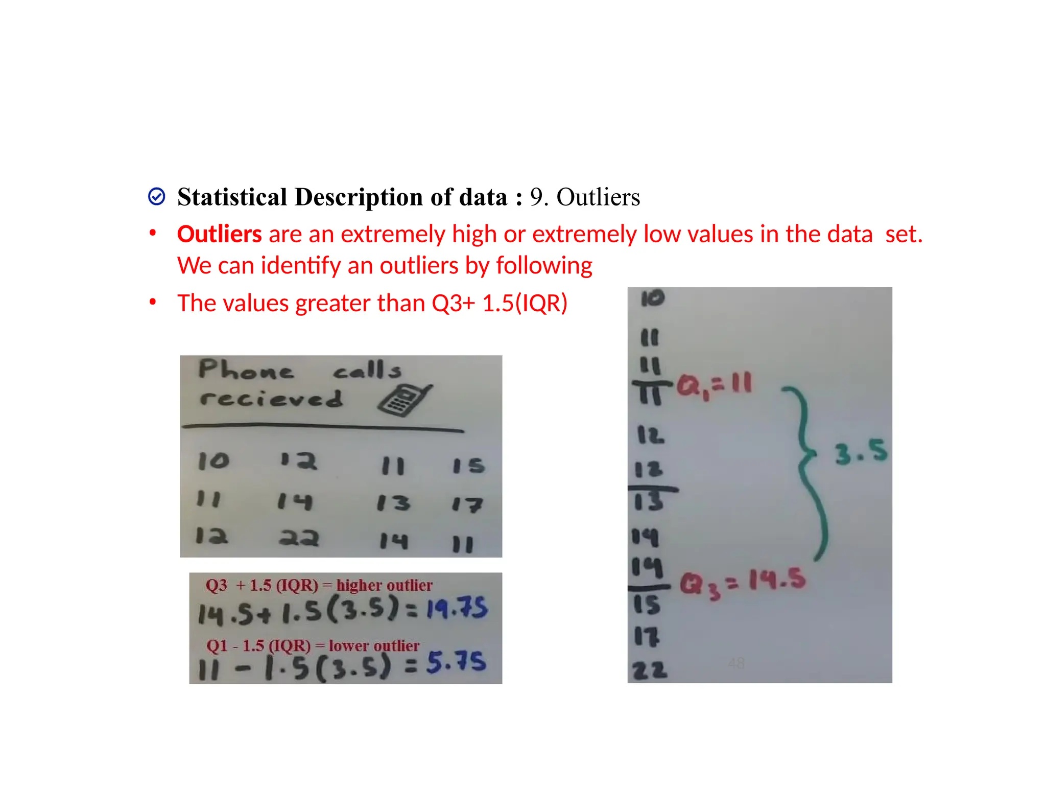
Statistical Description ofdata : 9. Outliers
• Outliers are an extremely high or extremely low values in the data set.
We can identify an outliers by following
• The values greater than Q3+ 1.5(IQR)
• The values less than Q1 – 1.5(IQR)
48
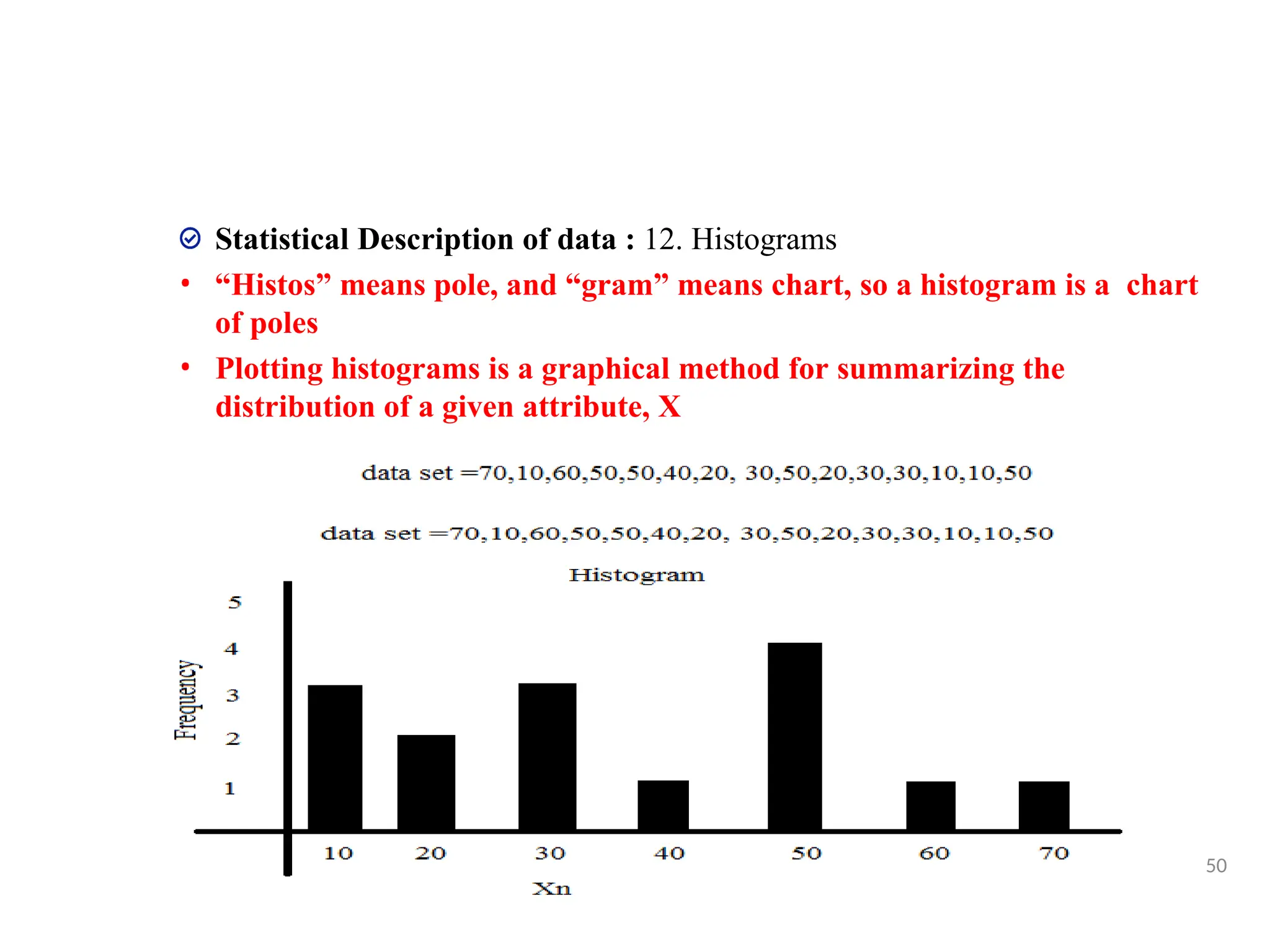
Statistical Description ofdata : 12. Histograms
• “Histos” means pole, and “gram” means chart, so a histogram is a chart
of poles
• Plotting histograms is a graphical method for summarizing the
distribution of a given attribute, X
50
51.
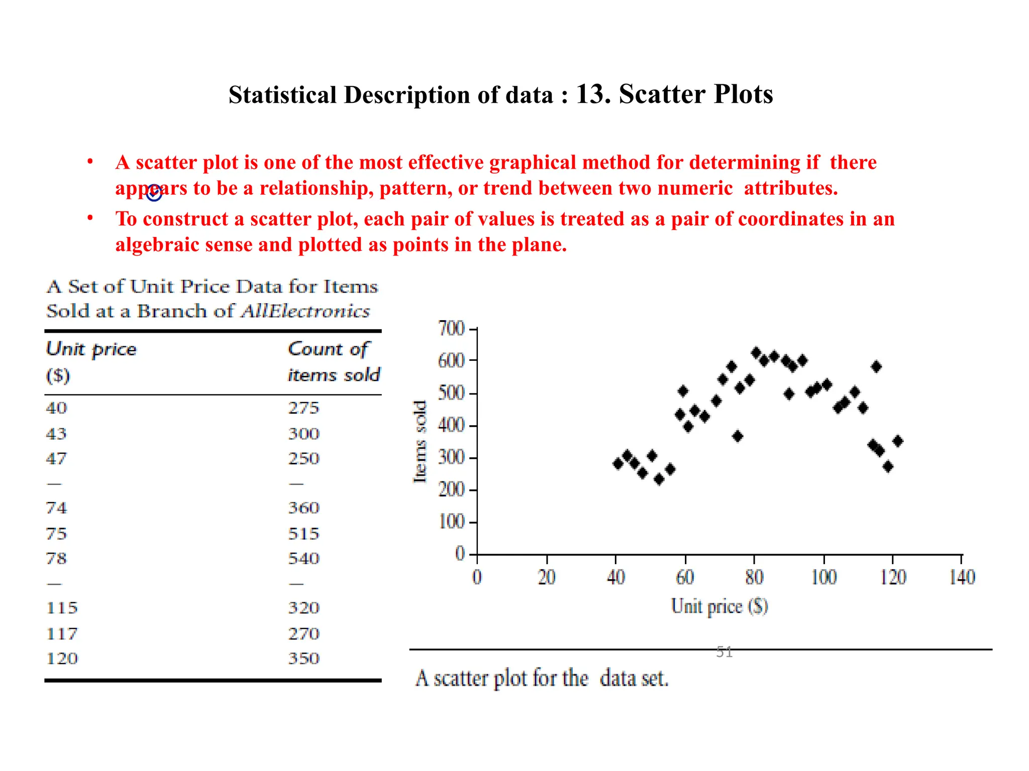
Statistical Description ofdata : 13. Scatter Plots
• A scatter plot is one of the most effective graphical method for determining if there
appears to be a relationship, pattern, or trend between two numeric attributes.
• To construct a scatter plot, each pair of values is treated as a pair of coordinates in an
algebraic sense and plotted as points in the plane.
51
52.
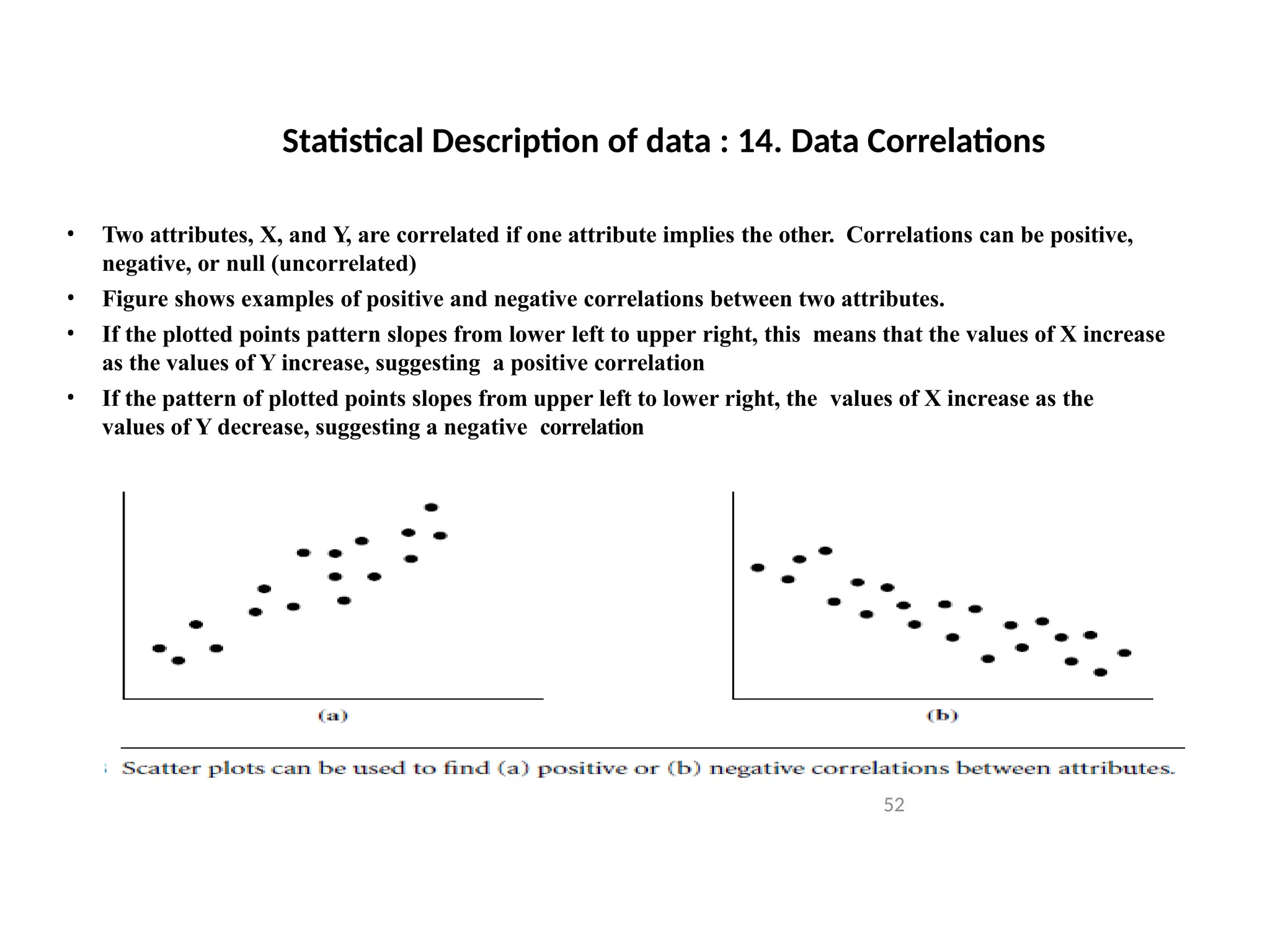
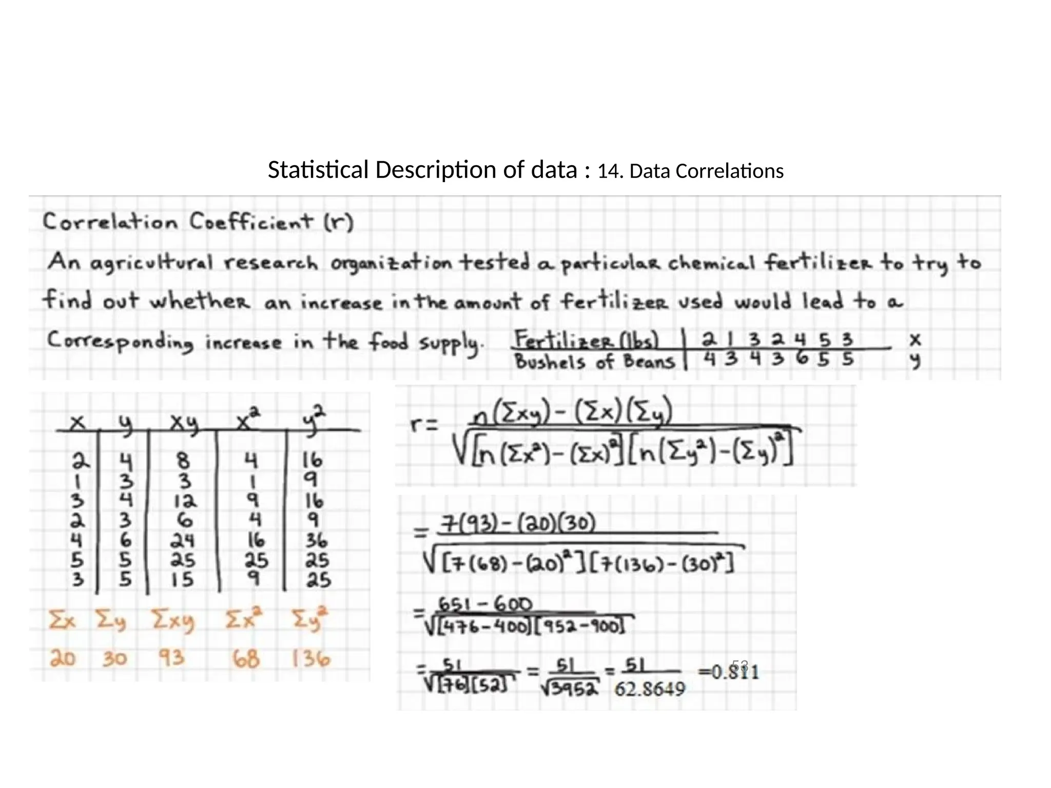
Statistical Description ofdata : 14. Data Correlations
• Two attributes, X, and Y, are correlated if one attribute implies the other. Correlations can be positive,
negative, or null (uncorrelated)
• Figure shows examples of positive and negative correlations between two attributes.
• If the plotted points pattern slopes from lower left to upper right, this means that the values of X increase
as the values of Y increase, suggesting a positive correlation
• If the pattern of plotted points slopes from upper left to lower right, the values of X increase as the
values of Y decrease, suggesting a negative correlation
52
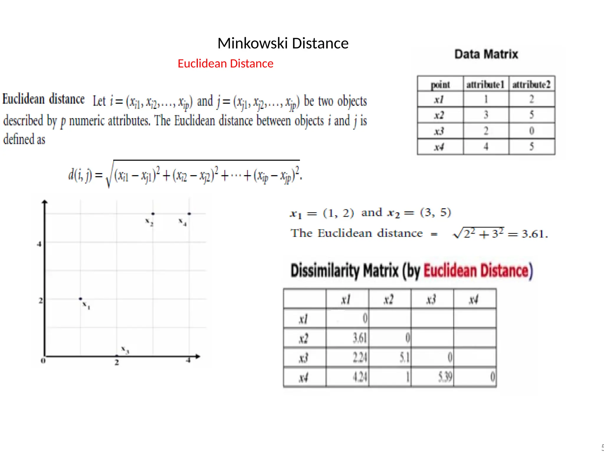
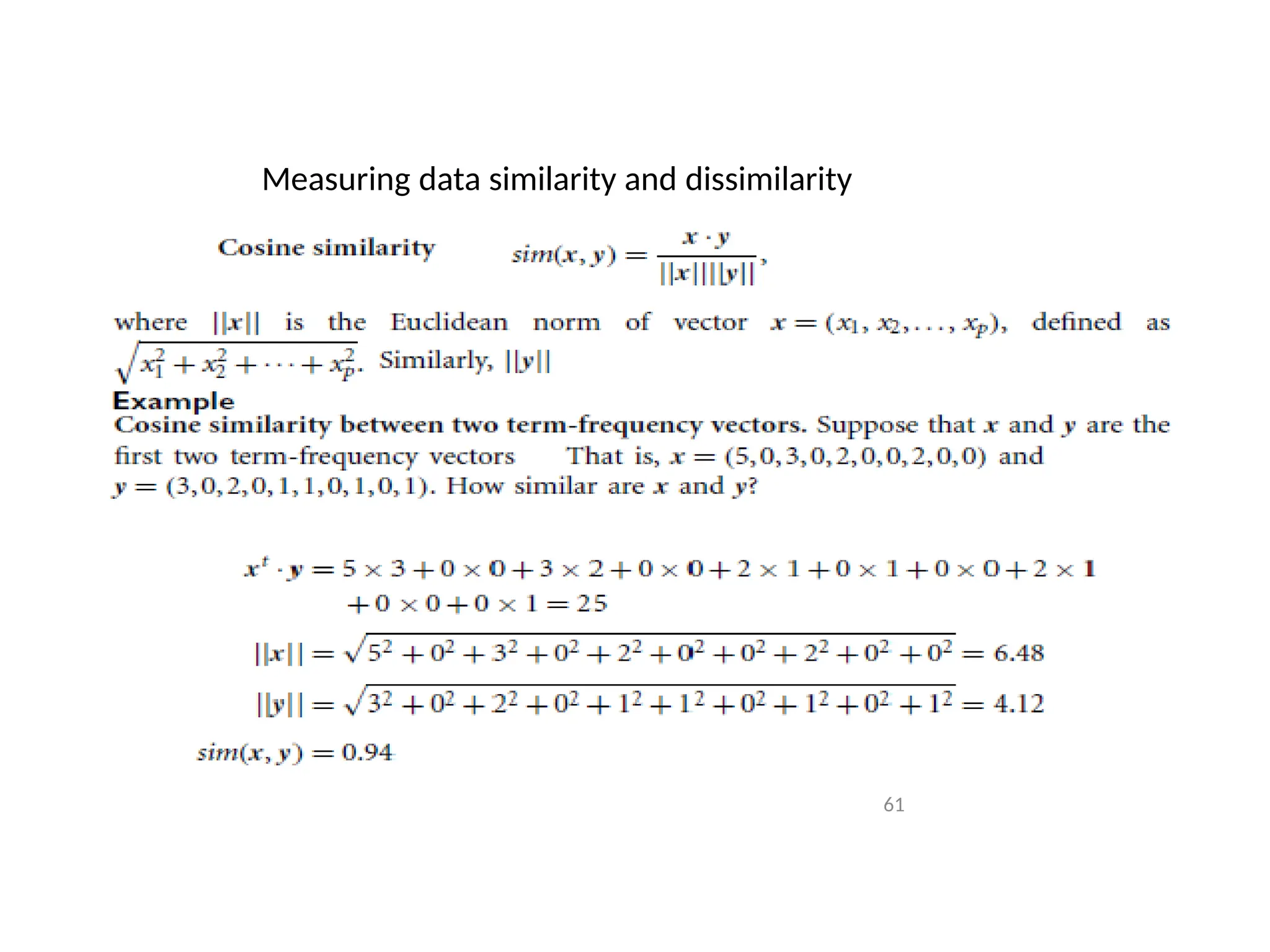
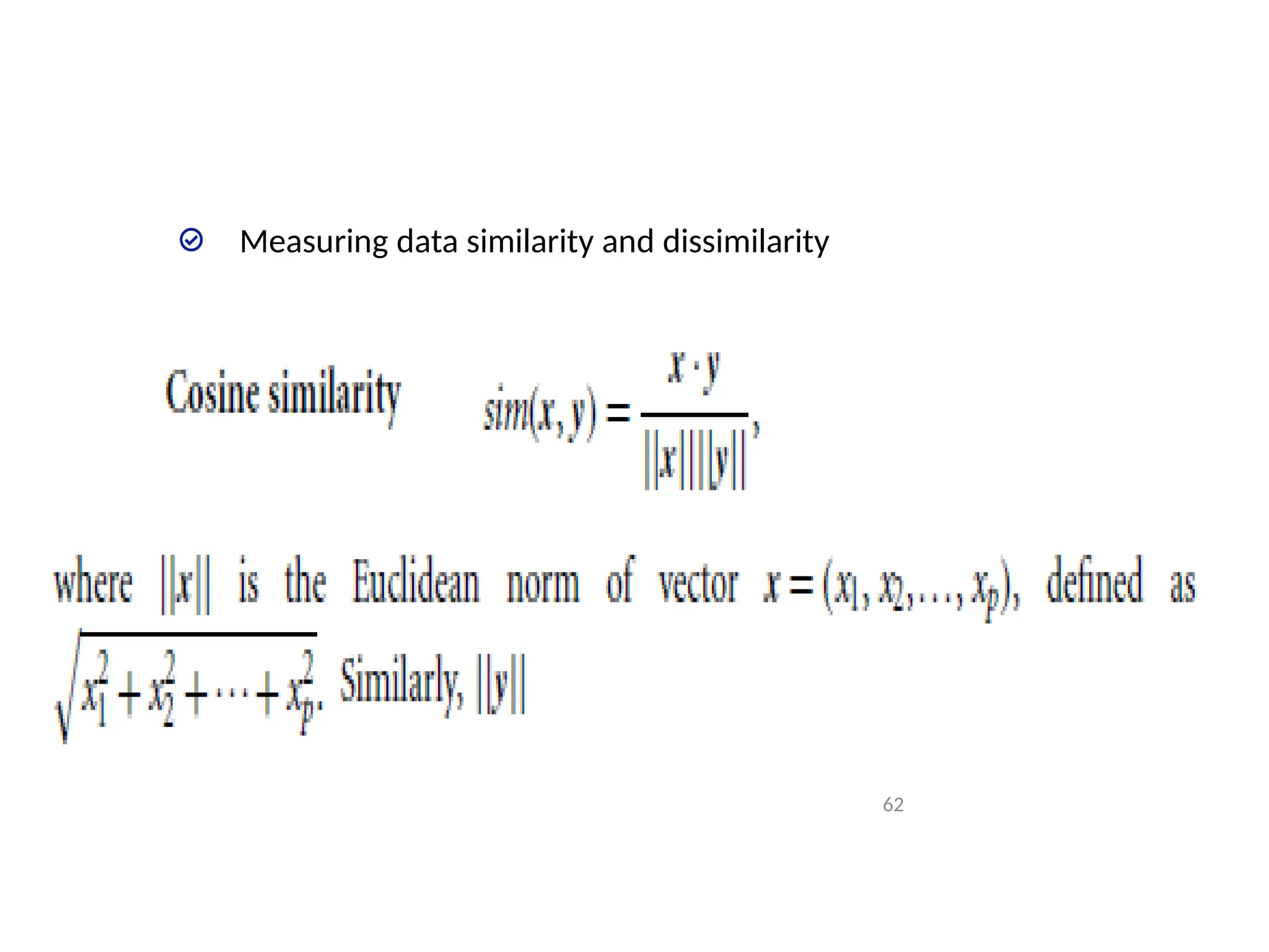
Measuring data similarityand dissimilarity
54
• In data mining applications(like clustering, classifications etc.) We are interested
in comparison of objects on the basis of their similarities and dissimilarities
• Similarities and dissimilarities can be measured by using following ways
1. Data Matrix
2. Dissimilarity Matrix
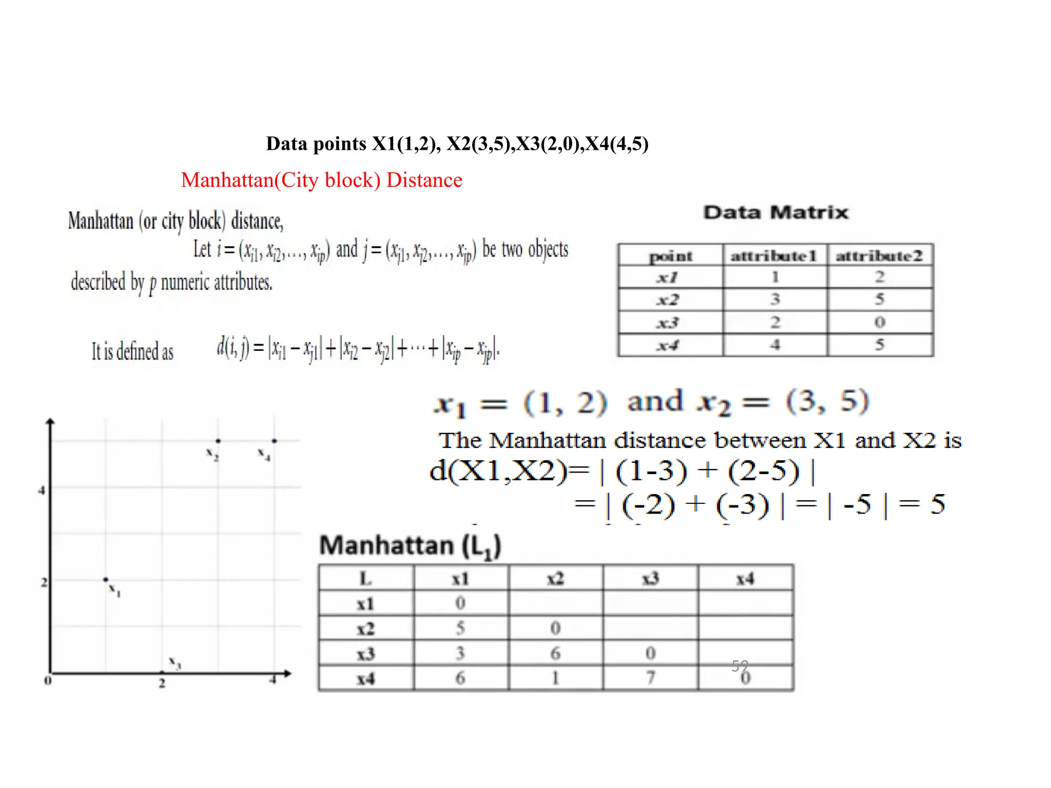
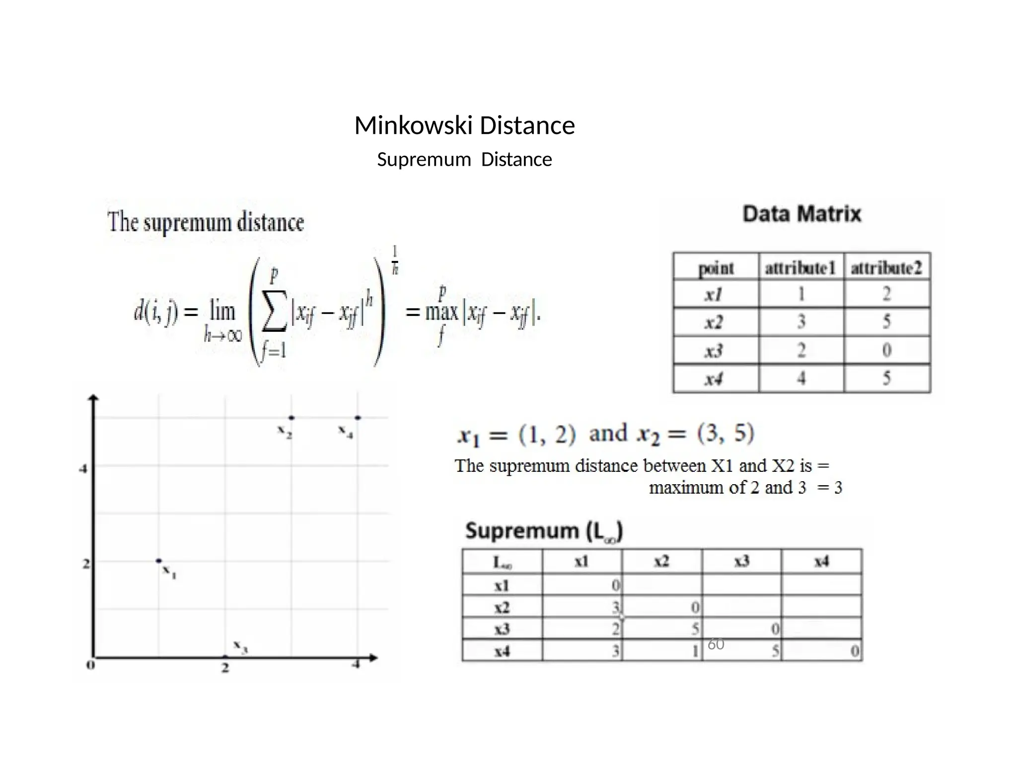
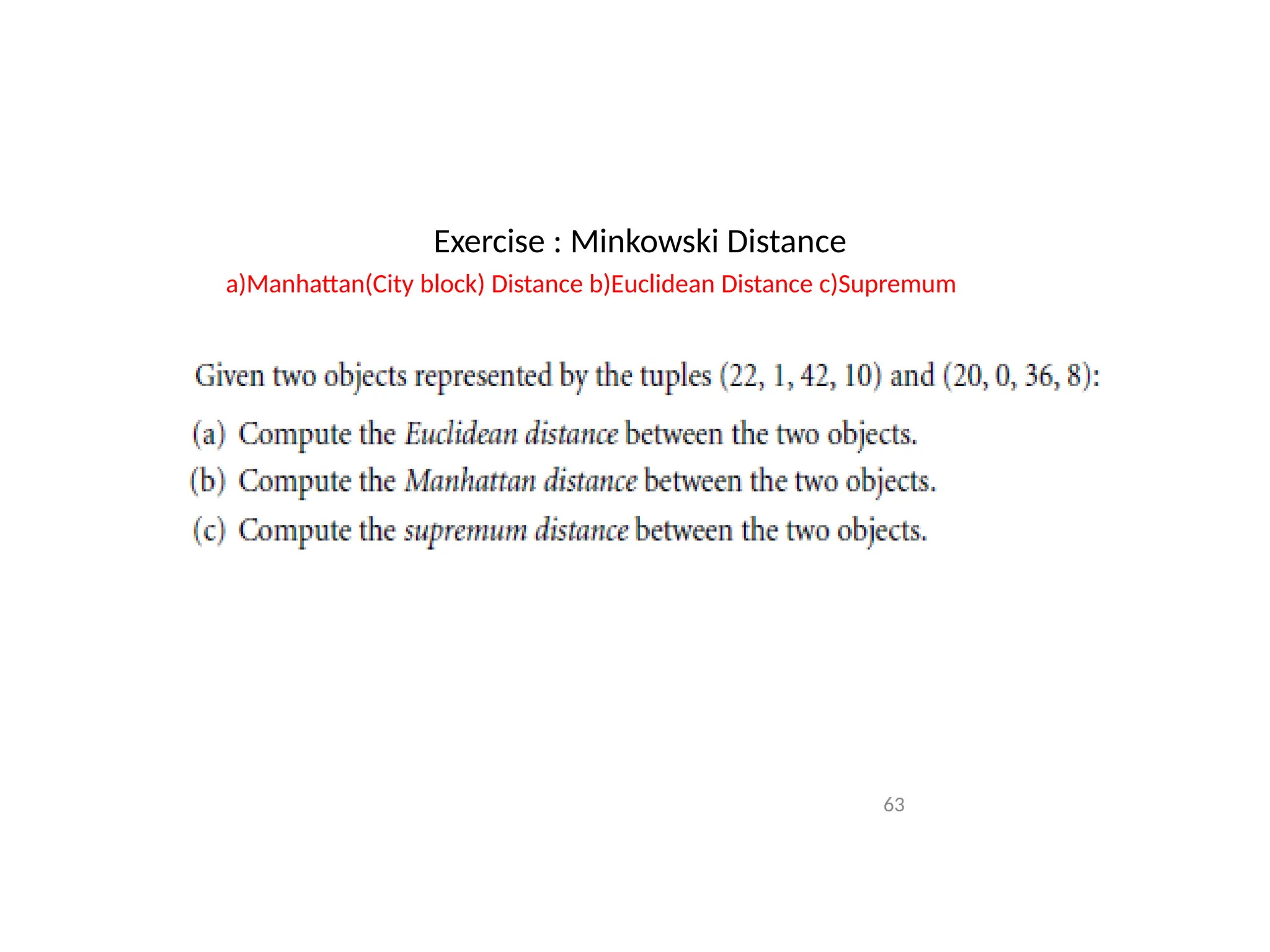
3. Minkowski Distance
a) Manhattan(City block) Distance
b) Euclidean Distance
c) Supremum Distance
4. Cosine similarity
55.
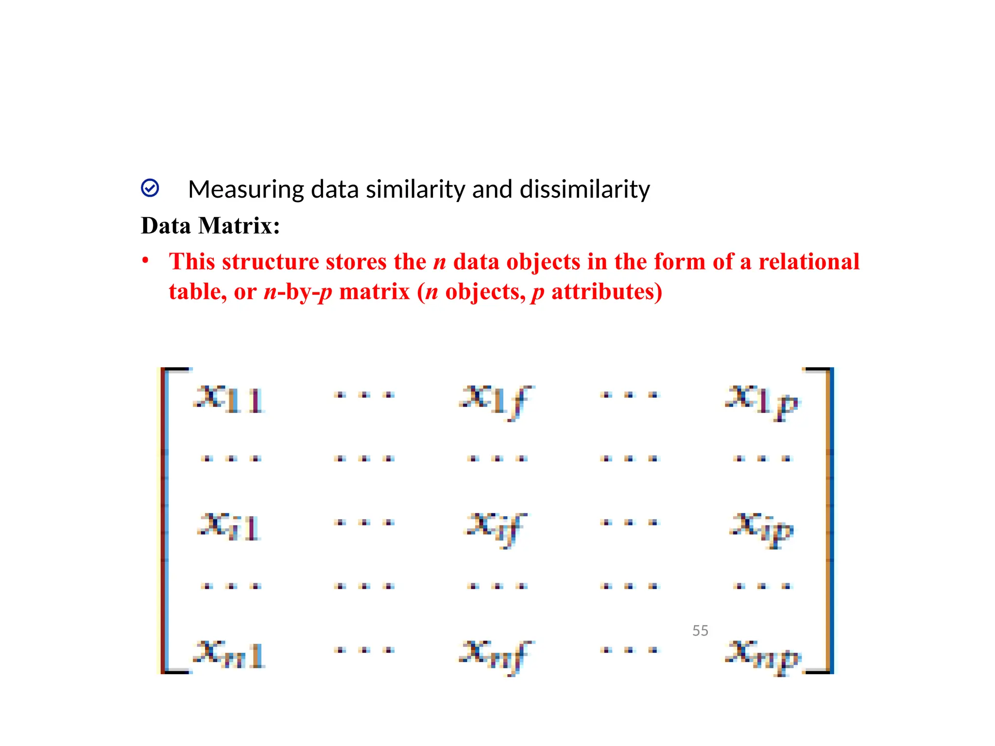
Measuring data similarityand dissimilarity
Data Matrix:
• This structure stores the n data objects in the form of a relational
table, or n-by-p matrix (n objects, p attributes)
55
56.
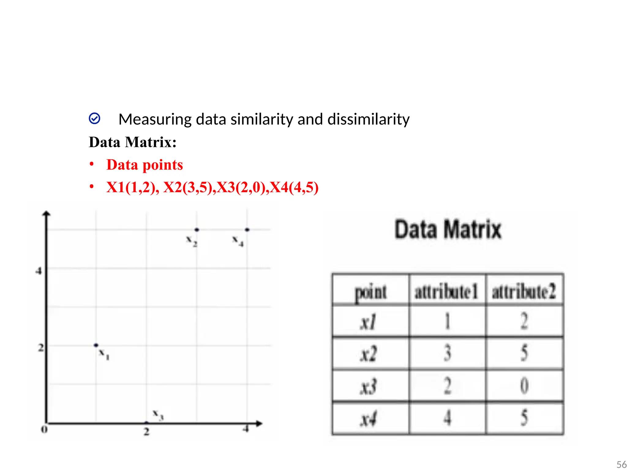
Measuring data similarityand dissimilarity
Data Matrix:
• Data points
• X1(1,2), X2(3,5),X3(2,0),X4(4,5)
56
57.
Measuring data similarityand dissimilarity
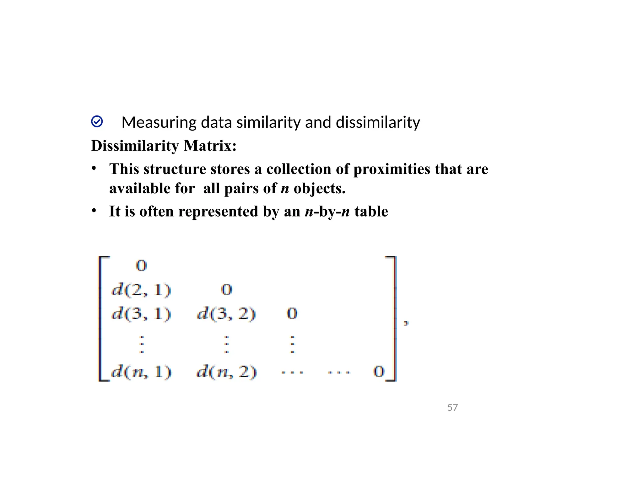
Dissimilarity Matrix:
• This structure stores a collection of proximities that are
available for all pairs of n objects.
• It is often represented by an n-by-n table
57
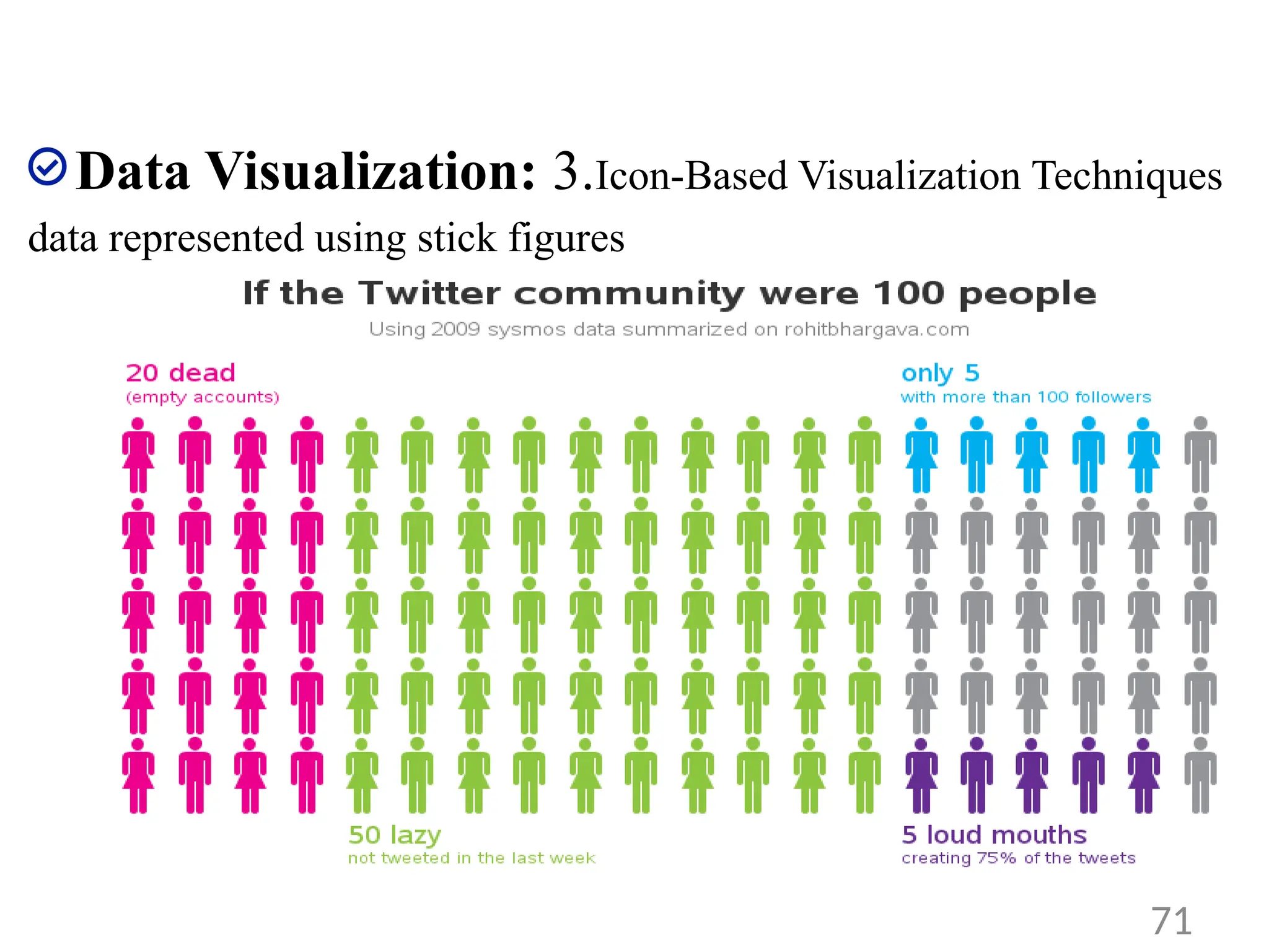
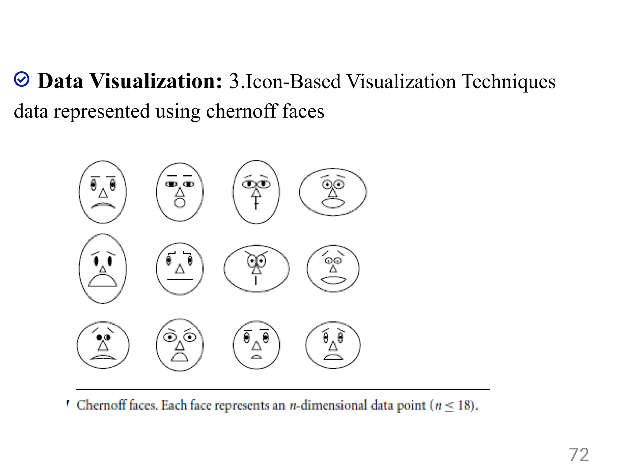
Data Visualization
• Datavisualization aims to communicate data clearly and
effectively through graphical representation.
• visualization techniques are used to discover data
relationships that are otherwise not easily observable by
looking at the raw data
• Data visualization techniques are divided into following types
1. Pixel-Oriented Visualization Techniques
2. Geometric Projection Visualization Techniques
3. Icon-Based Visualization Techniques
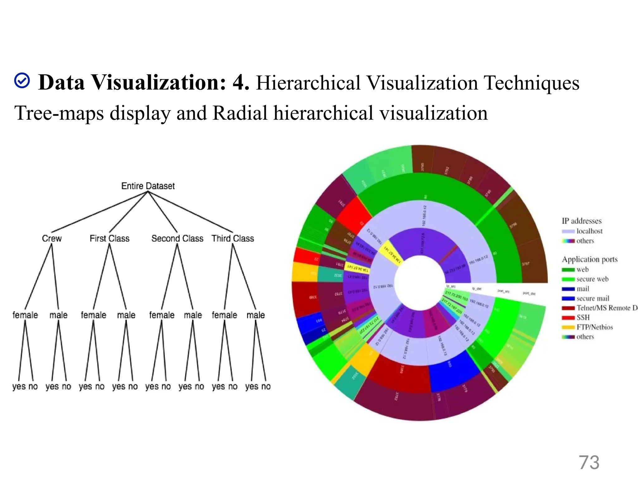
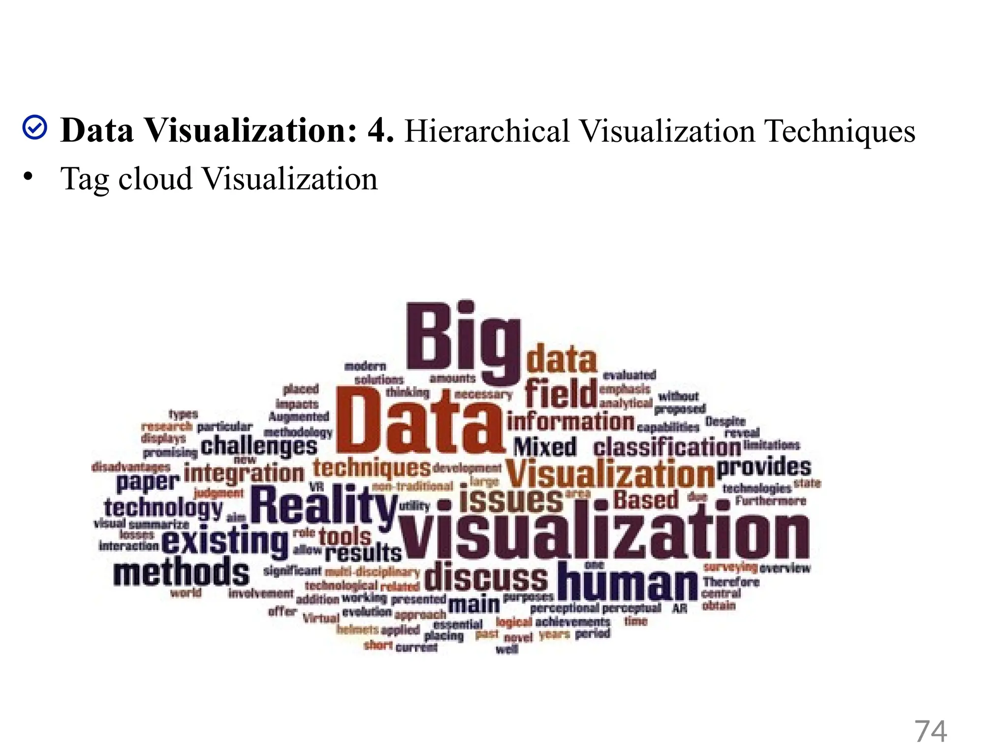
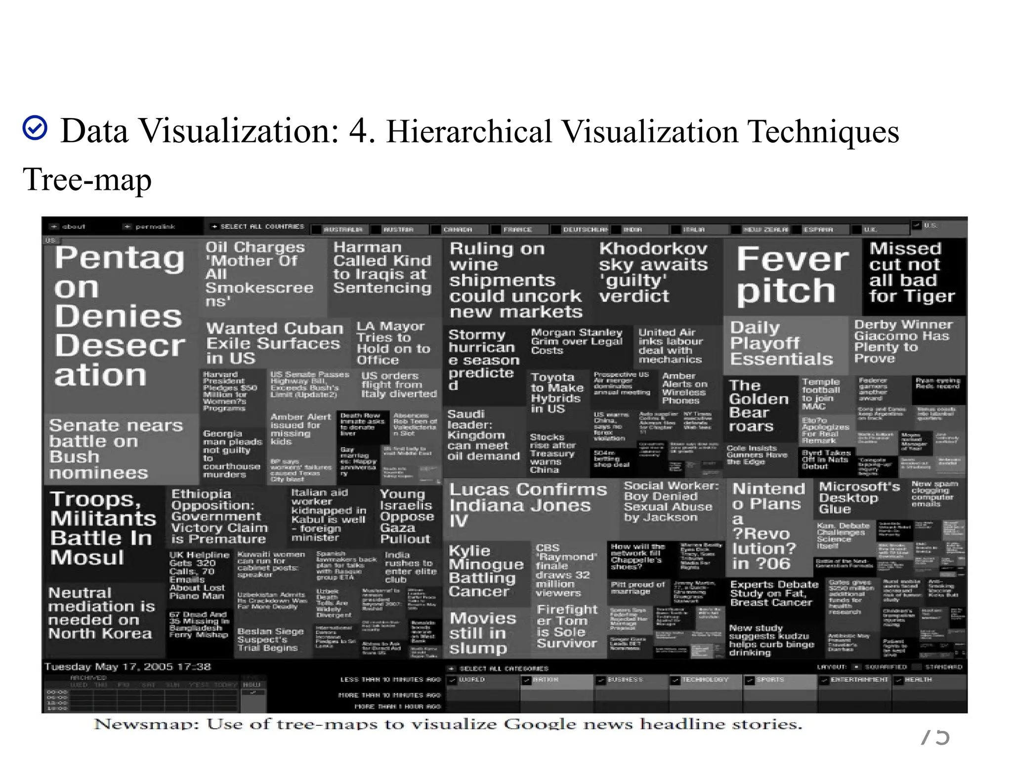
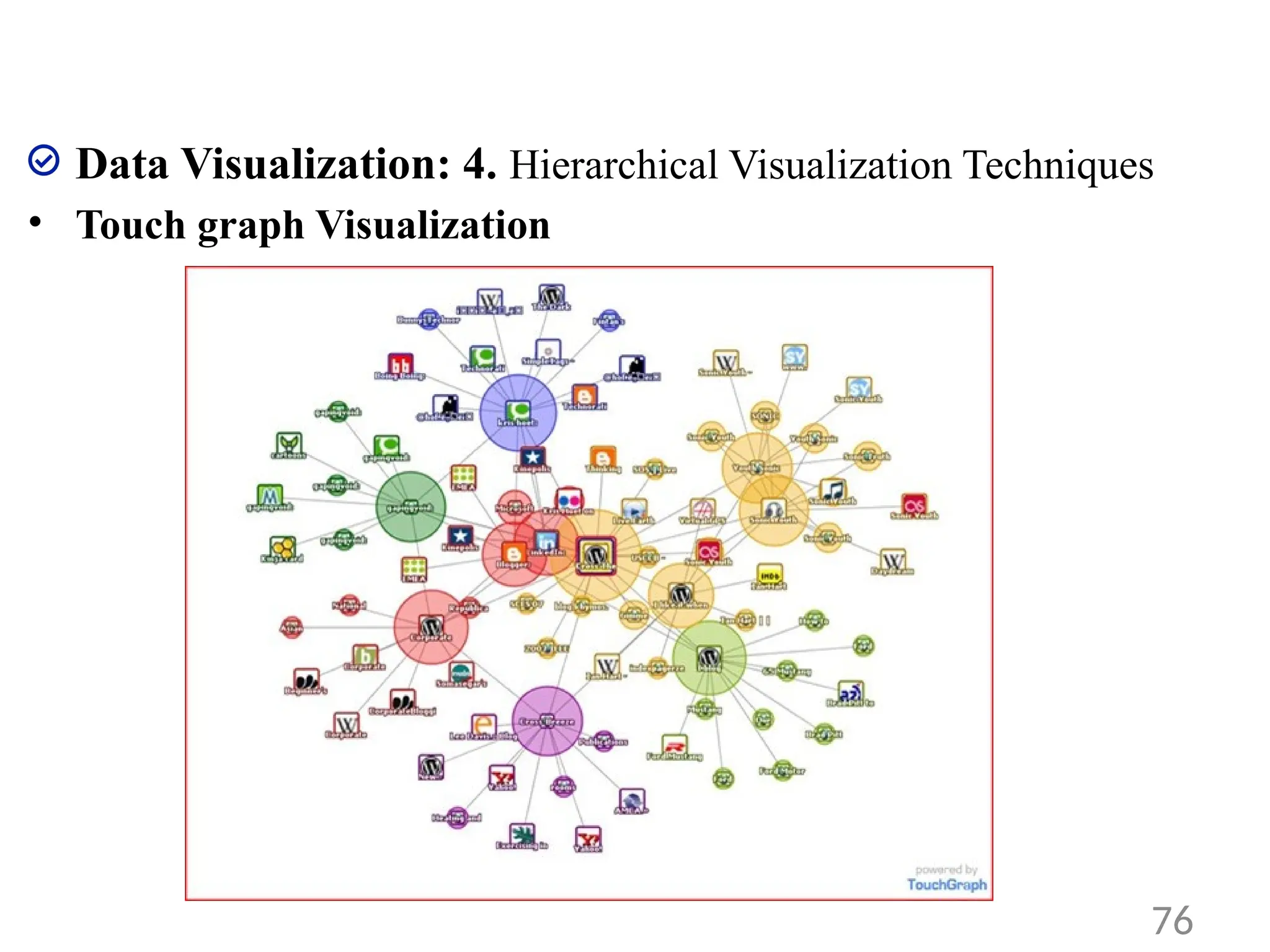
4. Hierarchical Visualization Techniques
64
65.
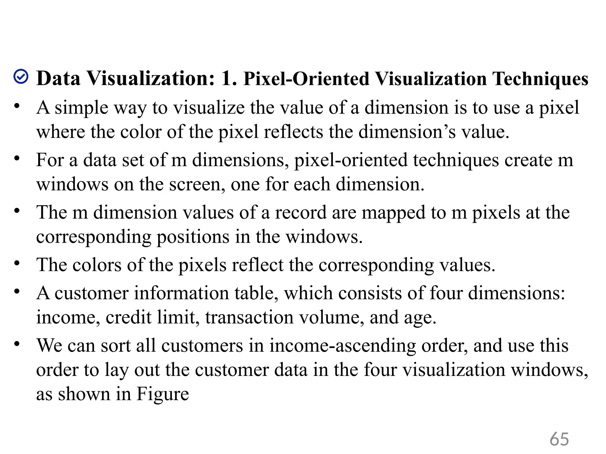
Data Visualization: 1.Pixel-Oriented Visualization Techniques
• A simple way to visualize the value of a dimension is to use a pixel
where the color of the pixel reflects the dimension’s value.
• For a data set of m dimensions, pixel-oriented techniques create m
windows on the screen, one for each dimension.
• The m dimension values of a record are mapped to m pixels at the
corresponding positions in the windows.
• The colors of the pixels reflect the corresponding values.
• A customer information table, which consists of four dimensions:
income, credit limit, transaction volume, and age.
• We can sort all customers in income-ascending order, and use this
order to lay out the customer data in the four visualization windows,
as shown in Figure
65
66.
Data Visualization: 1.Pixel-Oriented Visualization Techniques
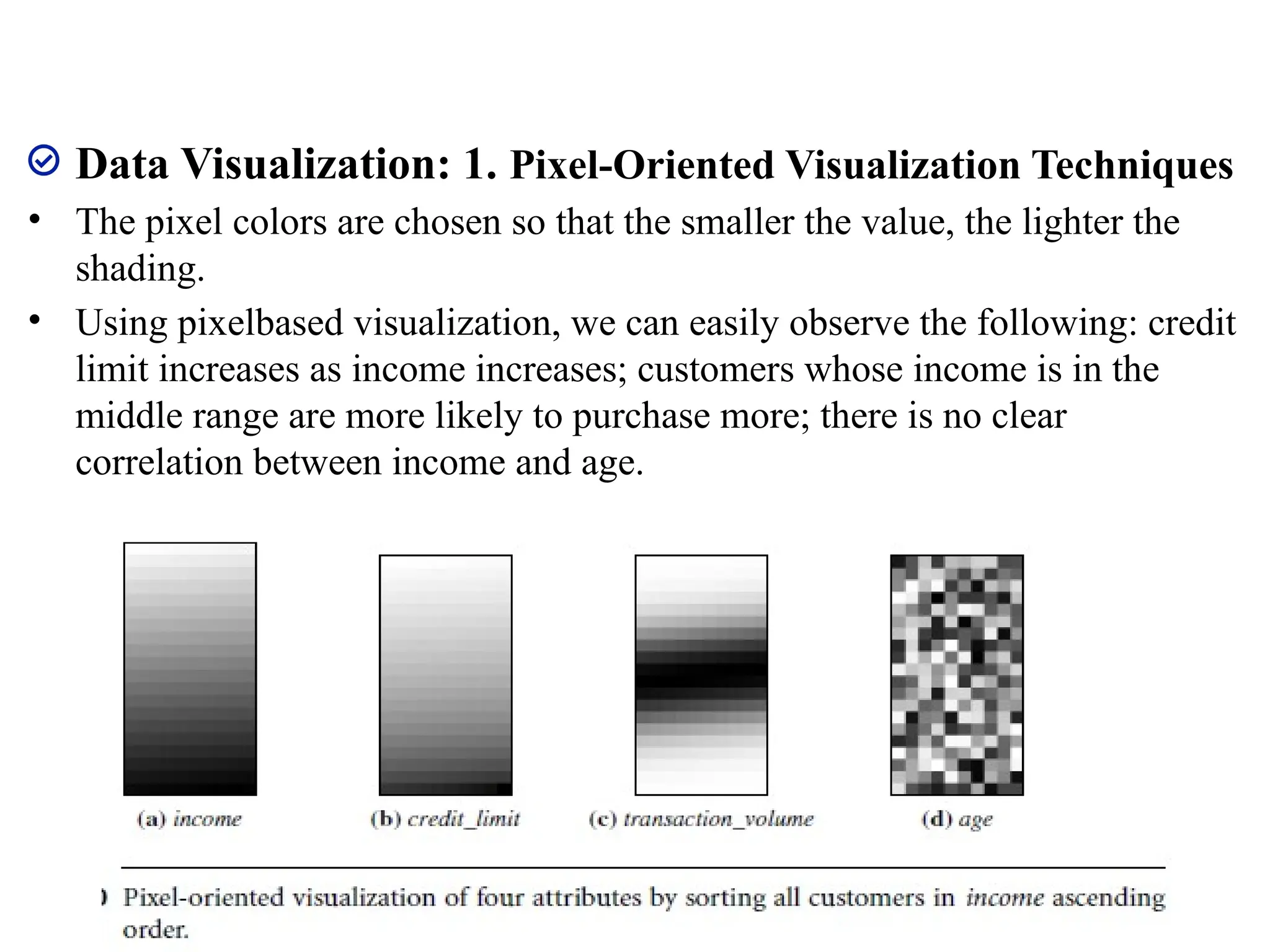
• The pixel colors are chosen so that the smaller the value, the lighter the
shading.
• Using pixelbased visualization, we can easily observe the following: credit
limit increases as income increases; customers whose income is in the
middle range are more likely to purchase more; there is no clear
correlation between income and age.
66
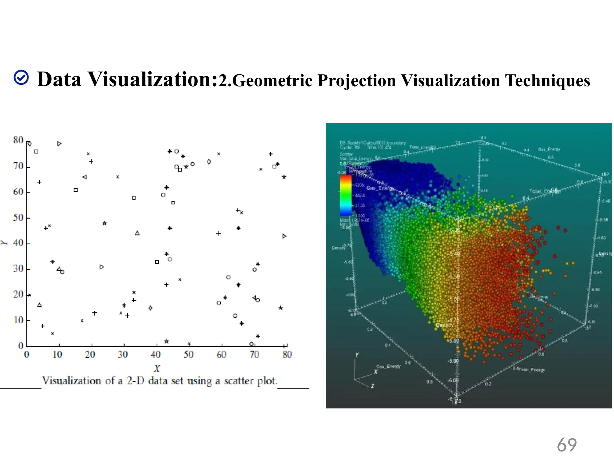
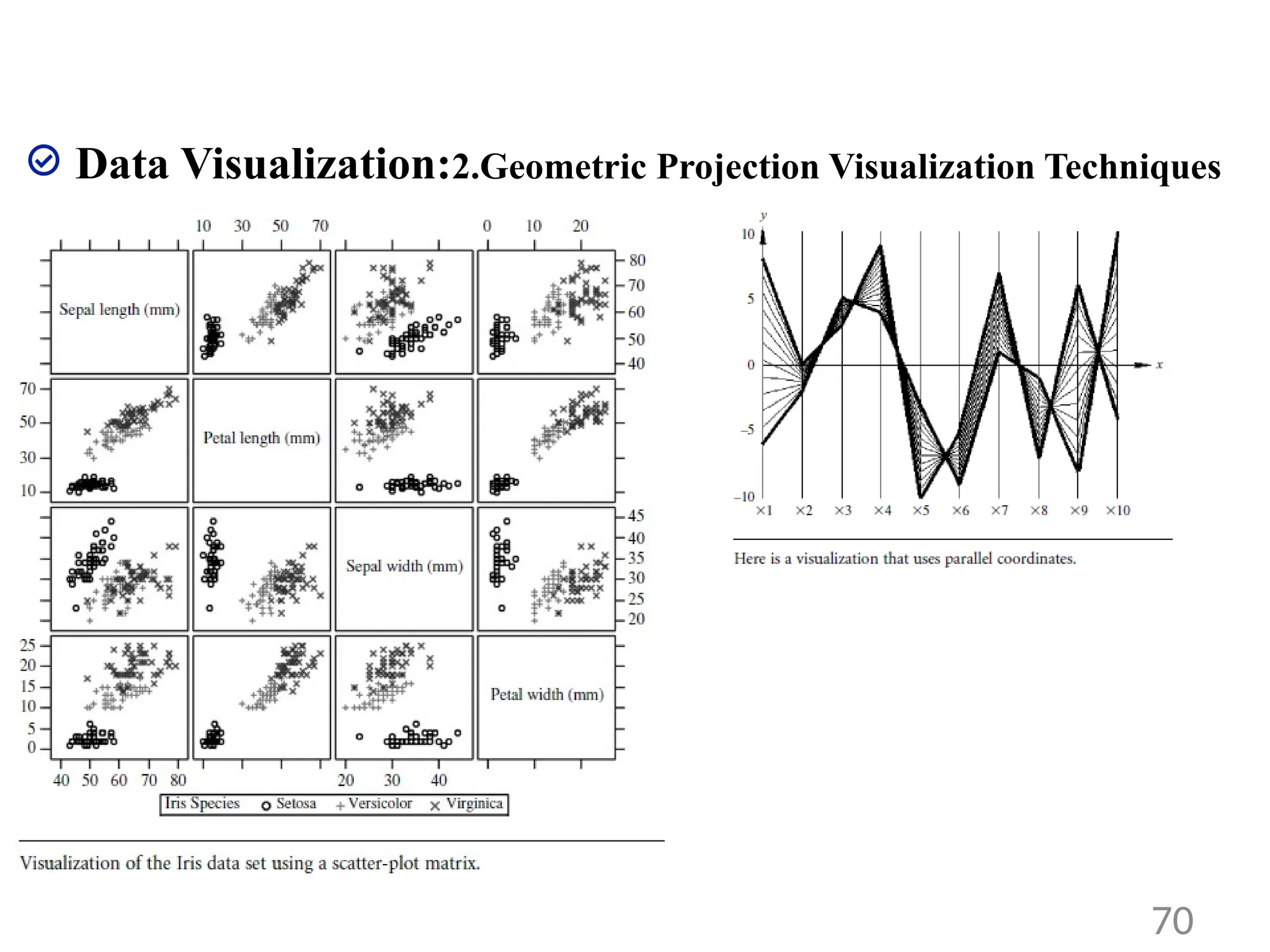
Data Visualization: 2.GeometricProjection Visualization
Techniques
• Geometric projection techniques help users find
interesting projections of multidimensional data sets.
• Figure shows an example, where X and Y are two spatial
attributes and the third dimension is represented by
different shapes.
• Through this visualization, we can see that points of types
“+” and “×” tend to be co located.
• A 3-D scatter plot uses three axes in a Cartesian coordinate
system. If it uses color, it can display up to 4-D data points
68
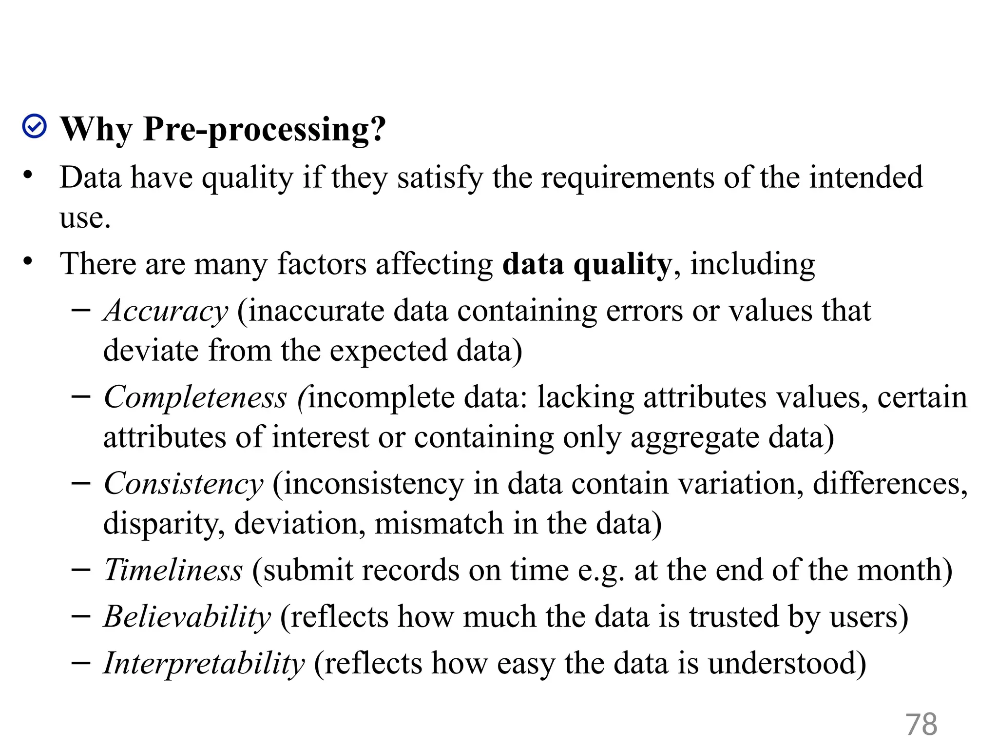
Why Pre-processing?
• Datahave quality if they satisfy the requirements of the intended
use.
• There are many factors affecting data quality, including
– Accuracy (inaccurate data containing errors or values that
deviate from the expected data)
– Completeness (incomplete data: lacking attributes values, certain
attributes of interest or containing only aggregate data)
– Consistency (inconsistency in data contain variation, differences,
disparity, deviation, mismatch in the data)
– Timeliness (submit records on time e.g. at the end of the month)
– Believability (reflects how much the data is trusted by users)
– Interpretability (reflects how easy the data is understood)
78
79.
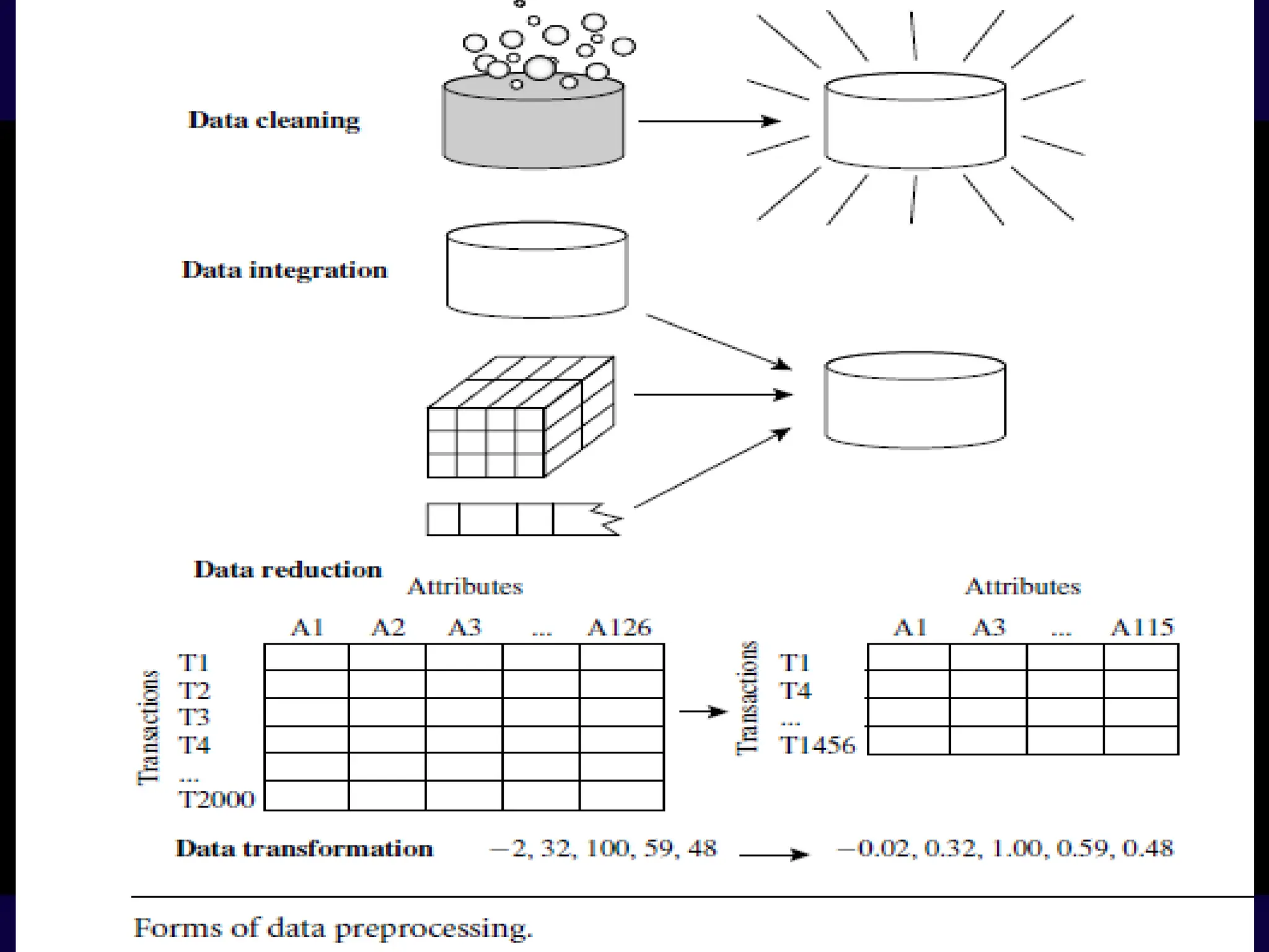
Major Tasks involvedin Data Preprocessing
• Following are the major steps involved in data preprocessing
• Data Cleaning
• Data Integration
• Data Reduction
• Data Transformation.
79
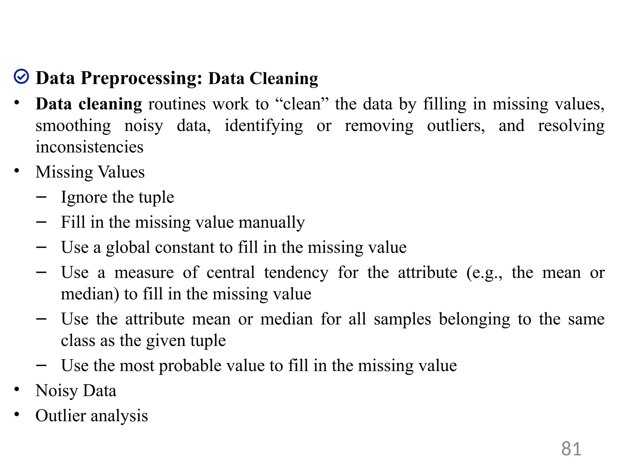
Data Preprocessing: DataCleaning
• Data cleaning routines work to “clean” the data by filling in missing values,
smoothing noisy data, identifying or removing outliers, and resolving
inconsistencies
• Missing Values
– Ignore the tuple
– Fill in the missing value manually
– Use a global constant to fill in the missing value
– Use a measure of central tendency for the attribute (e.g., the mean or
median) to fill in the missing value
– Use the attribute mean or median for all samples belonging to the same
class as the given tuple
– Use the most probable value to fill in the missing value
• Noisy Data
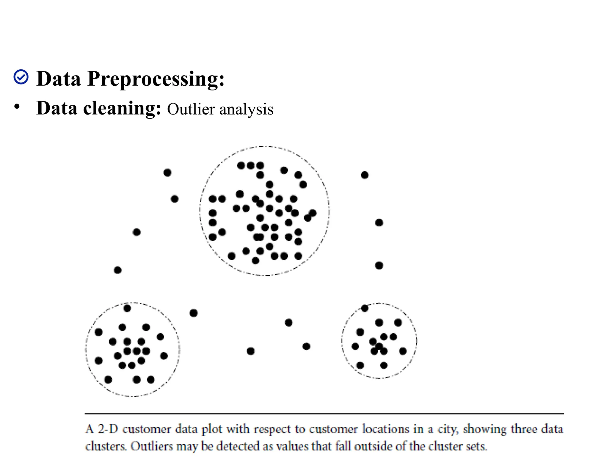
• Outlier analysis
81
Data Preprocessing:
• Dataintegration: this involve integrating multiple databases, data
cubes, or files
• combines data from multiple sources to form a coherent data store.
• following concepts contribute to smooth data integration.
– The resolution of semantic heterogeneity
– metadata
– correlation analysis
– tuple duplication detection
– data conflict detection
83
84.
Data Preprocessing: DataReduction
• Data reduction obtains a reduced representation of the data set that
is much smaller in volume, yet produces the same (or almost the
same) analytical results.
• Data reduction strategies include
– data cube aggregation
– dimensionality reduction
– data compression
– numerosity reduction.
84
85.
Data Preprocessing: DataReduction
• Data cube aggregation, where aggregation operations are applied to
the data in the construction of data cube.
• In dimensionality reduction, data encoding schemes are applied so
as to obtain a reduced or “compressed” representation of the original
data (e.g., removing irrelevant attributes)
• Data compression, where encoding mechanisms are used to reduce
the data set size
• In numerosity reduction, the data are replaced by alternative,
smaller representations using parametric models (e.g., regression or
log-linear models) or nonparametric models (e.g., histograms,
clusters, sampling, or data aggregation)
85
86.
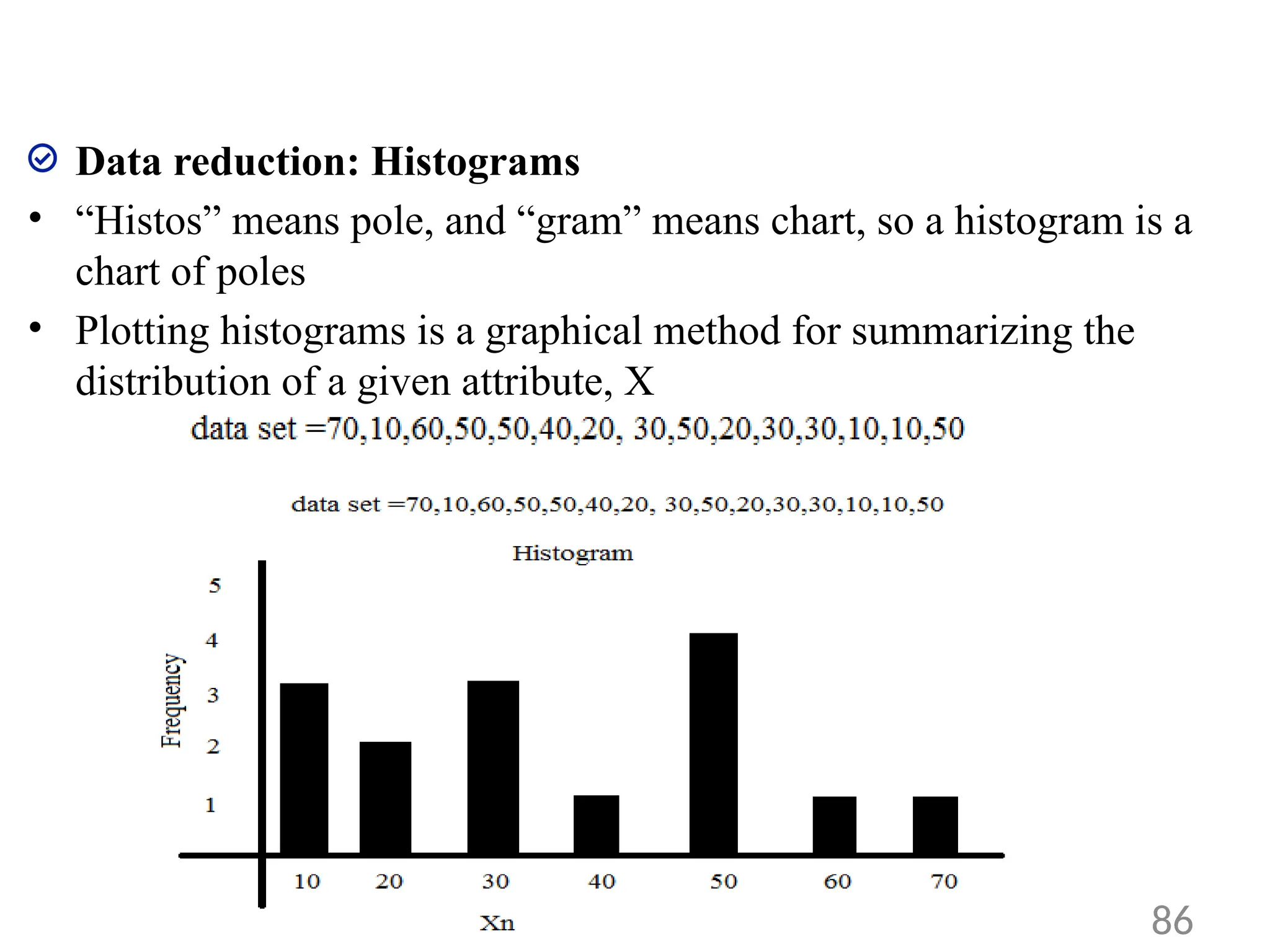
Data reduction: Histograms
•“Histos” means pole, and “gram” means chart, so a histogram is a
chart of poles
• Plotting histograms is a graphical method for summarizing the
distribution of a given attribute, X
86
87.
Data Preprocessing: Datareduction
Attribute subset selection
• Attribute subset selection is a method of dimensionality reduction in
which irrelevant, weakly relevant, or redundant attributes or
dimensions are detected and removed
• The goal of attribute subset selection is to find a minimum set of
attributes such that the resulting probability distribution of the data
classes is as close as possible to the original distribution obtained
using all attributes
• It reduces the number of attributes appearing in the discovered
patterns, helping to make the patterns easier to understand.
87
88.
Data Preprocessing: Datareduction
Clustering and sampling
• Clustering techniques consider data tuples as objects. They partition
the objects into groups, or clusters, so that objects within a cluster
are “similar” to one another and “dissimilar” to objects in other
clusters.
• Sampling can be used as a data reduction technique because it
allows a large data set to be represented by a much smaller random
data sample (or subset)
88
89.
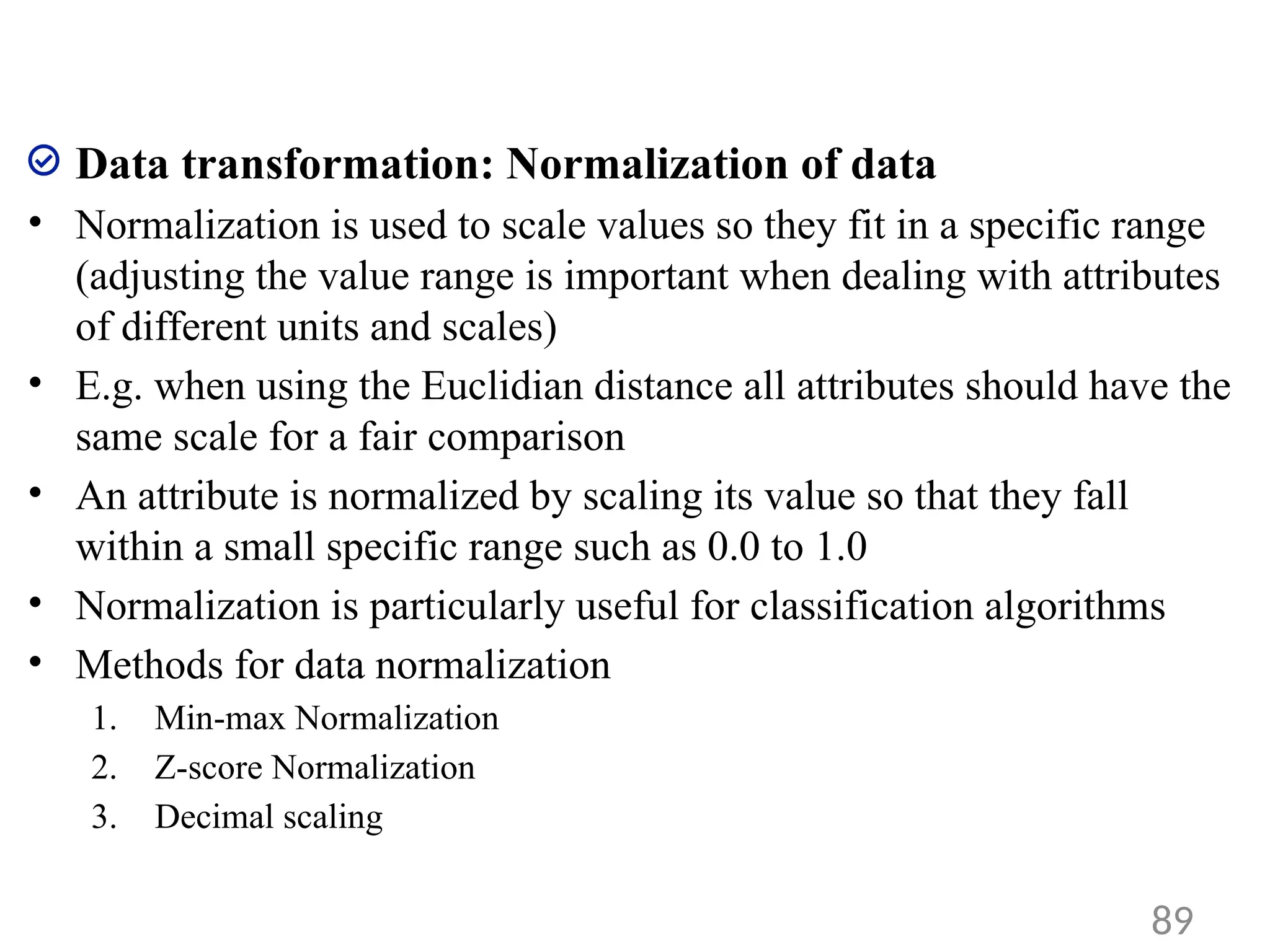
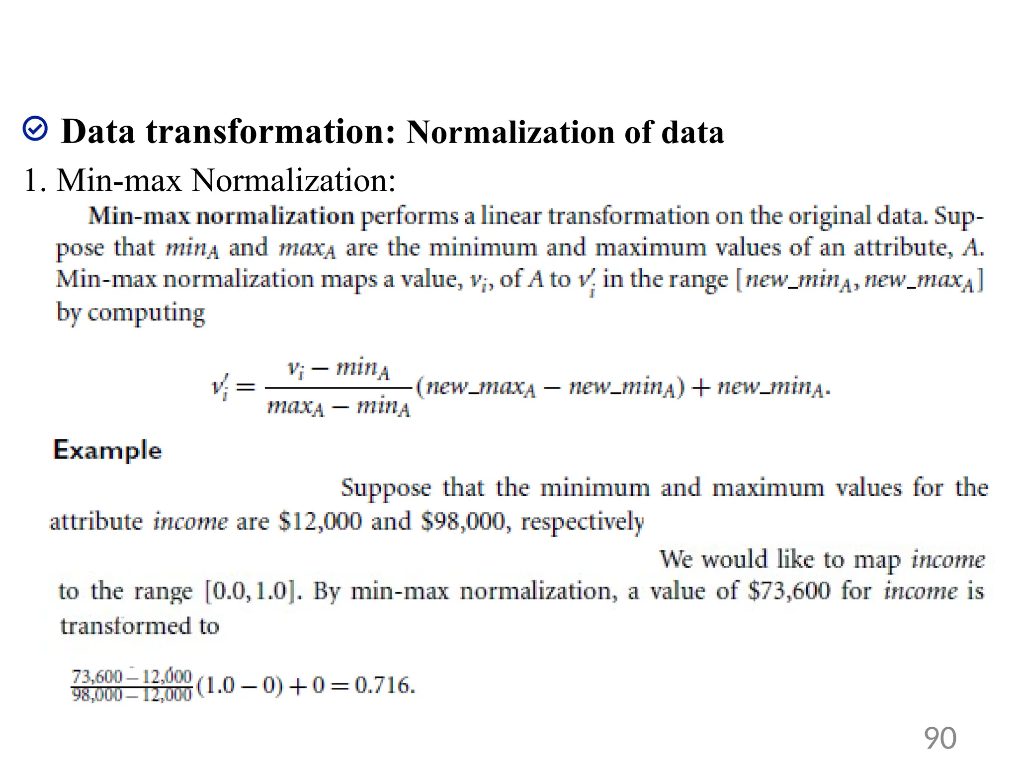
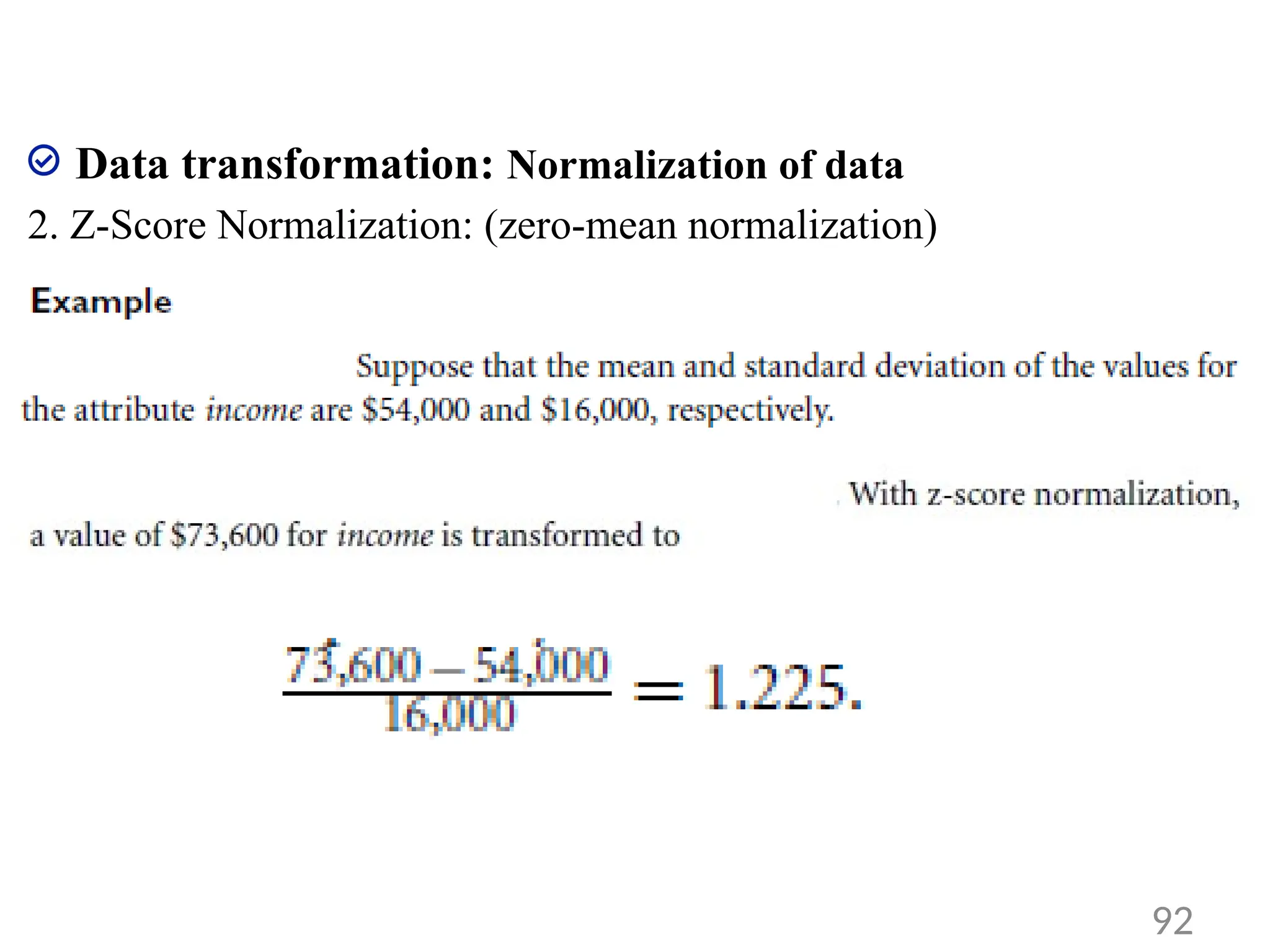
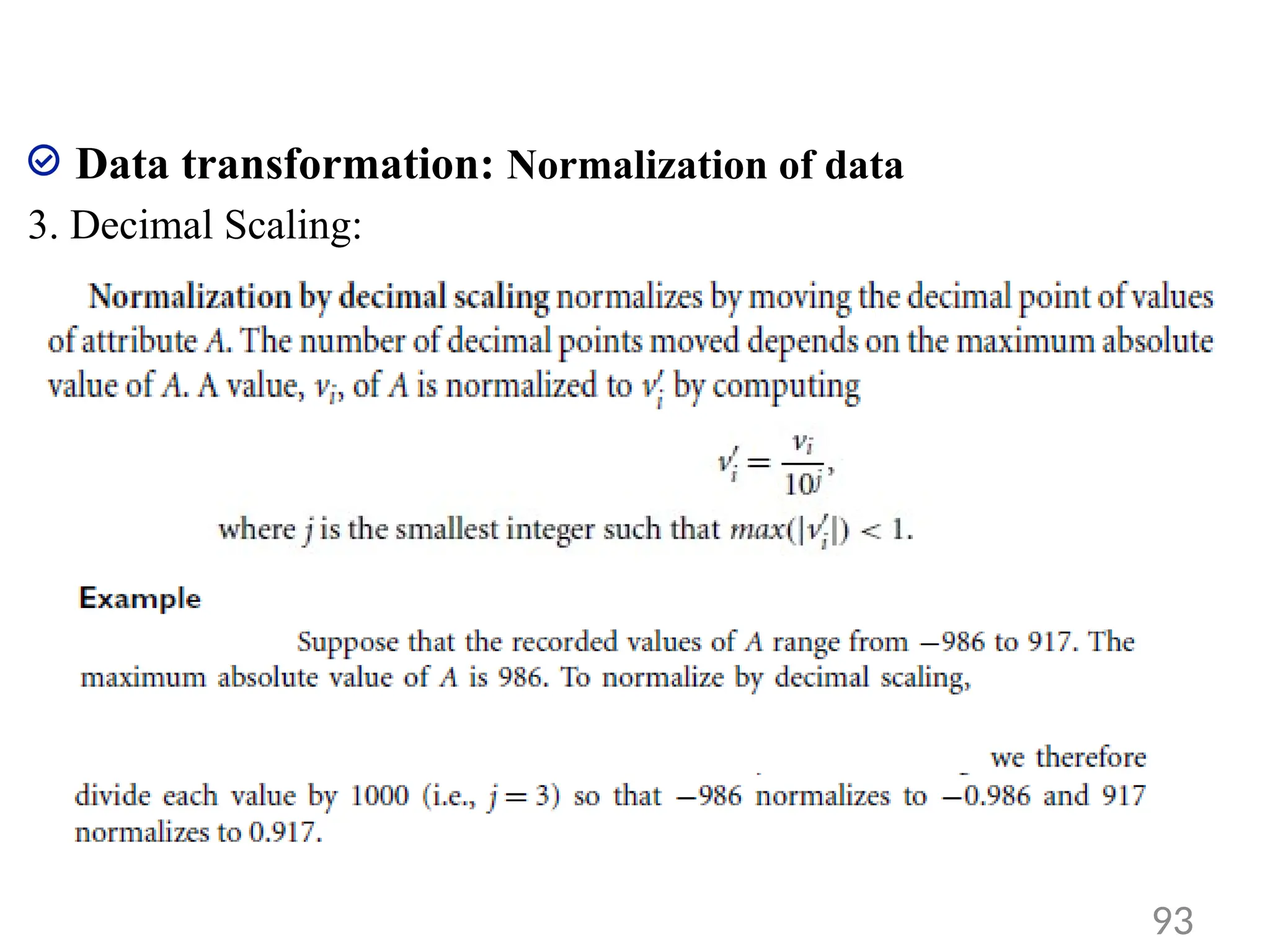
Data transformation: Normalizationof data
• Normalization is used to scale values so they fit in a specific range
(adjusting the value range is important when dealing with attributes
of different units and scales)
• E.g. when using the Euclidian distance all attributes should have the
same scale for a fair comparison
• An attribute is normalized by scaling its value so that they fall
within a small specific range such as 0.0 to 1.0
• Normalization is particularly useful for classification algorithms
• Methods for data normalization
1. Min-max Normalization
2. Z-score Normalization
3. Decimal scaling
89
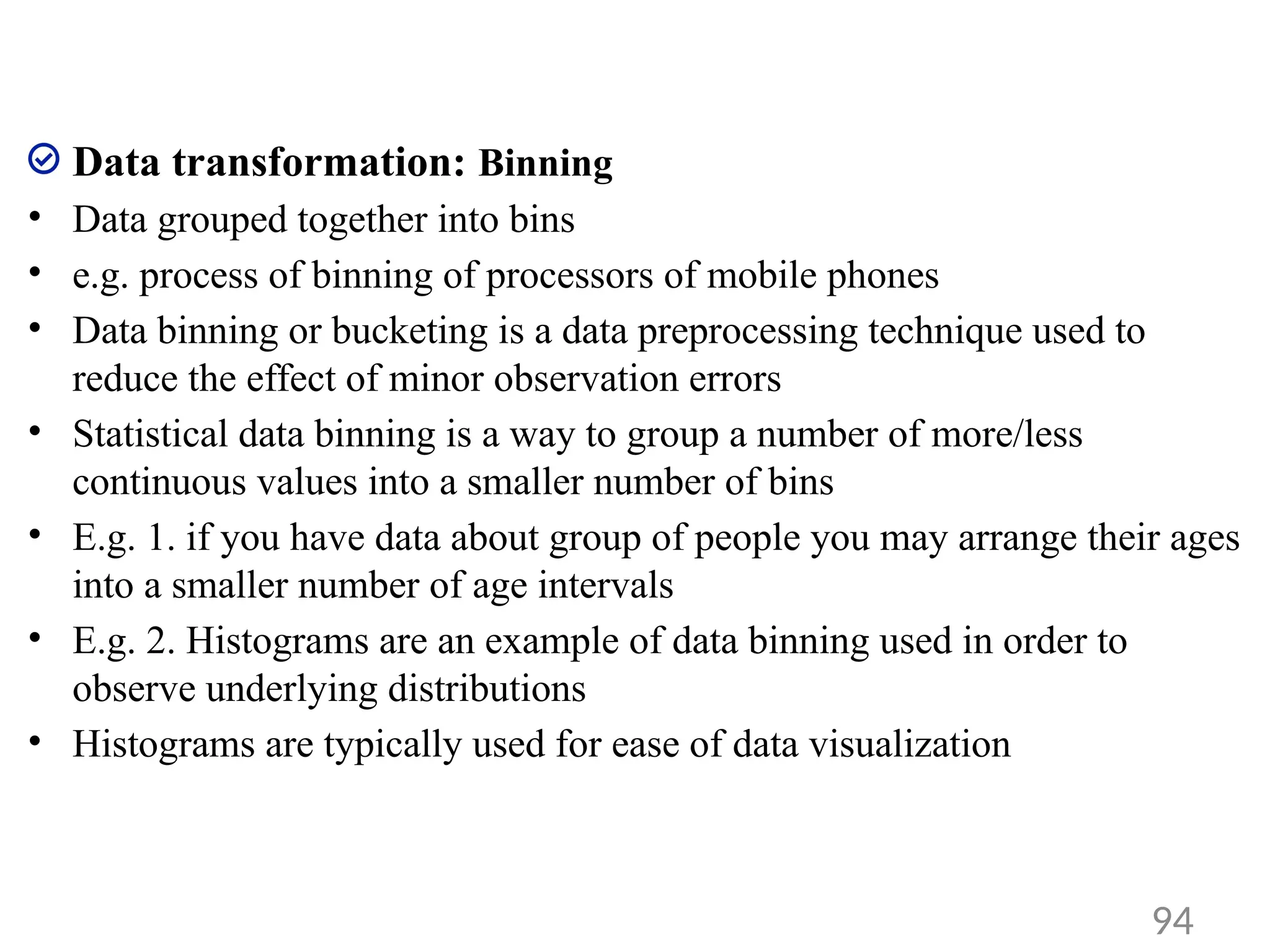
Data transformation: Binning
•Data grouped together into bins
• e.g. process of binning of processors of mobile phones
• Data binning or bucketing is a data preprocessing technique used to
reduce the effect of minor observation errors
• Statistical data binning is a way to group a number of more/less
continuous values into a smaller number of bins
• E.g. 1. if you have data about group of people you may arrange their ages
into a smaller number of age intervals
• E.g. 2. Histograms are an example of data binning used in order to
observe underlying distributions
• Histograms are typically used for ease of data visualization
94
95.
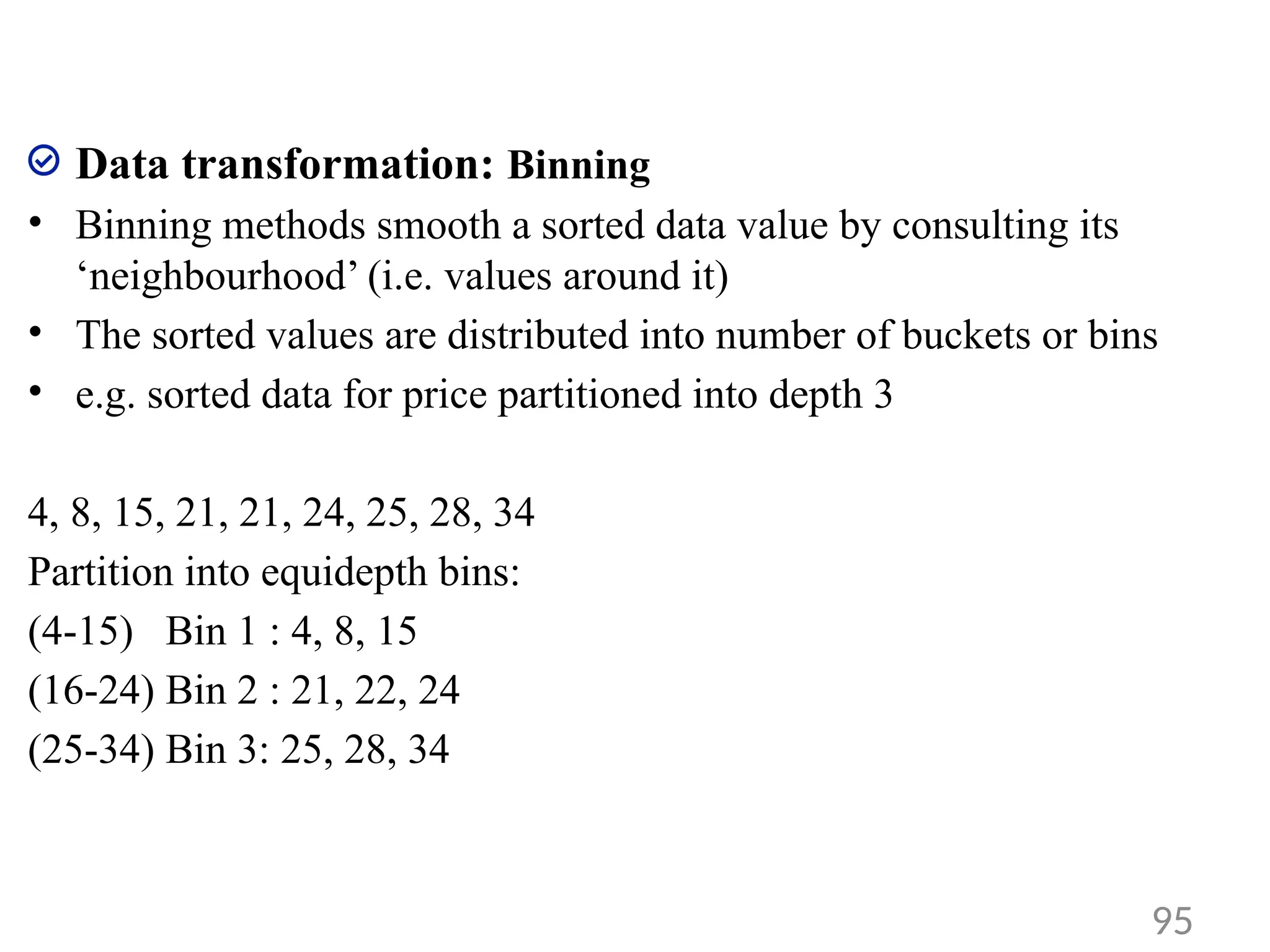
Data transformation: Binning
•Binning methods smooth a sorted data value by consulting its
‘neighbourhood’ (i.e. values around it)
• The sorted values are distributed into number of buckets or bins
• e.g. sorted data for price partitioned into depth 3
4, 8, 15, 21, 21, 24, 25, 28, 34
Partition into equidepth bins:
(4-15) Bin 1 : 4, 8, 15
(16-24) Bin 2 : 21, 22, 24
(25-34) Bin 3: 25, 28, 34
95
96.
Data transformation: Binning
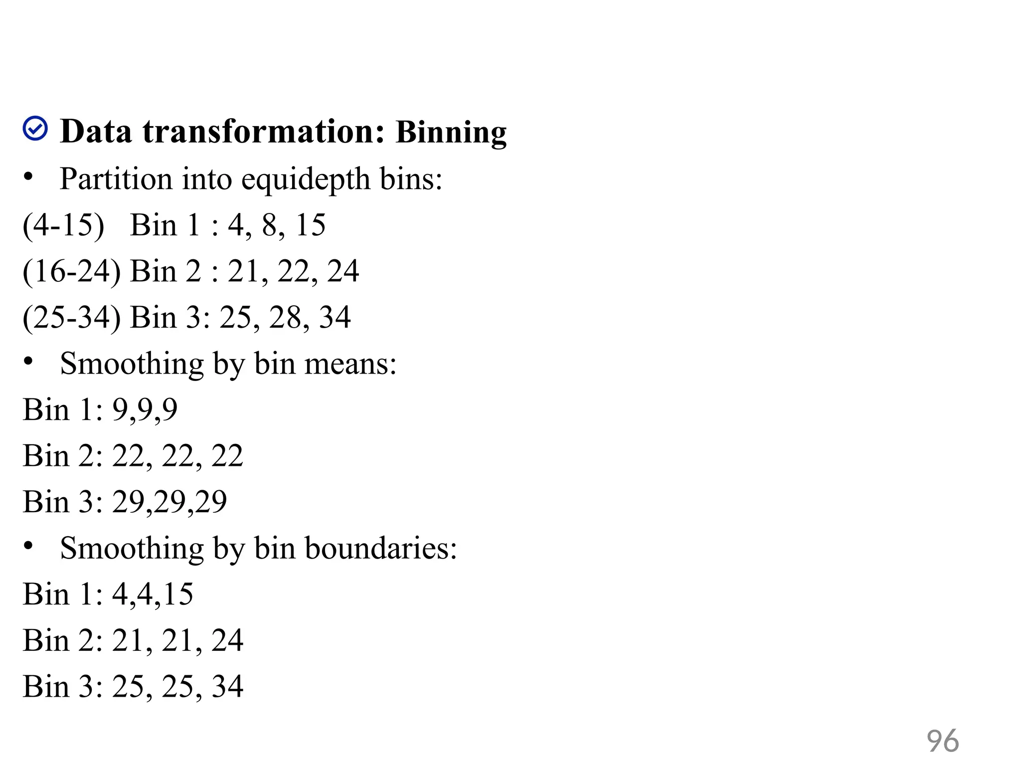
•Partition into equidepth bins:
(4-15) Bin 1 : 4, 8, 15
(16-24) Bin 2 : 21, 22, 24
(25-34) Bin 3: 25, 28, 34
• Smoothing by bin means:
Bin 1: 9,9,9
Bin 2: 22, 22, 22
Bin 3: 29,29,29
• Smoothing by bin boundaries:
Bin 1: 4,4,15
Bin 2: 21, 21, 24
Bin 3: 25, 25, 34
96
97.
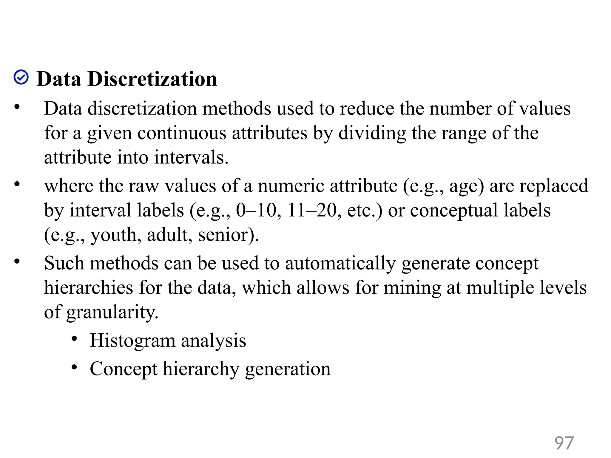
Data Discretization
• Datadiscretization methods used to reduce the number of values
for a given continuous attributes by dividing the range of the
attribute into intervals.
• where the raw values of a numeric attribute (e.g., age) are replaced
by interval labels (e.g., 0–10, 11–20, etc.) or conceptual labels
(e.g., youth, adult, senior).
• Such methods can be used to automatically generate concept
hierarchies for the data, which allows for mining at multiple levels
of granularity.
• Histogram analysis
• Concept hierarchy generation
97
98.
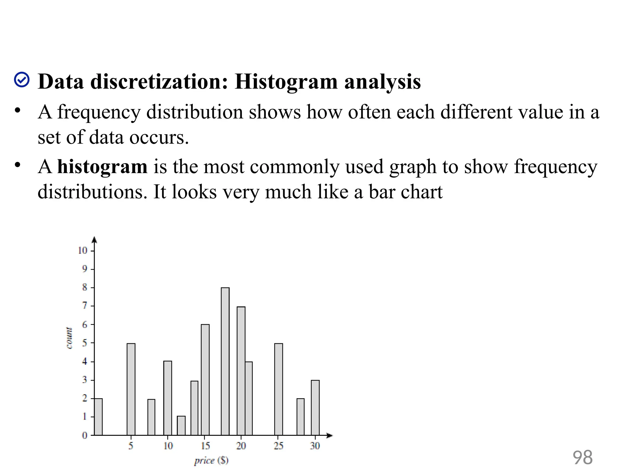
Data discretization: Histogramanalysis
• A frequency distribution shows how often each different value in a
set of data occurs.
• A histogram is the most commonly used graph to show frequency
distributions. It looks very much like a bar chart
98
99.
Data discretization: Concepthierarchy generation
• The concept hierarchies can be used to transform the data into
multiple levels of granularity
• four methods for the generation of concept hierarchies for nominal
data
1. Specification of a partial ordering of attributes explicitly at the schema level by
users or experts
2. Specification of a portion of a hierarchy by explicit data grouping
3. Specification of a set of attributes, but not of their partial ordering
4. Specification of only a partial set of attributes
99
100.
Data discretization: Concepthierarchy generation
1. Specification of a partial ordering of attributes explicitly at the
schema level by users or experts
• user or expert can easily define a concept hierarchy by specifying a
partial or total ordering of the attributes at the schema level.
• e.g. location dimension may contain the attributes (specifying the
ordering) such as street < city < province or state < country
2. Specification of a portion of a hierarchy by explicit data grouping
• a user could define some intermediate levels manually
• E.g. {ABC road, Hyderabad, A.P, India} subset of South India
• {XYZ road, Amritsar, Punjab, India} subset of North India
100
101.
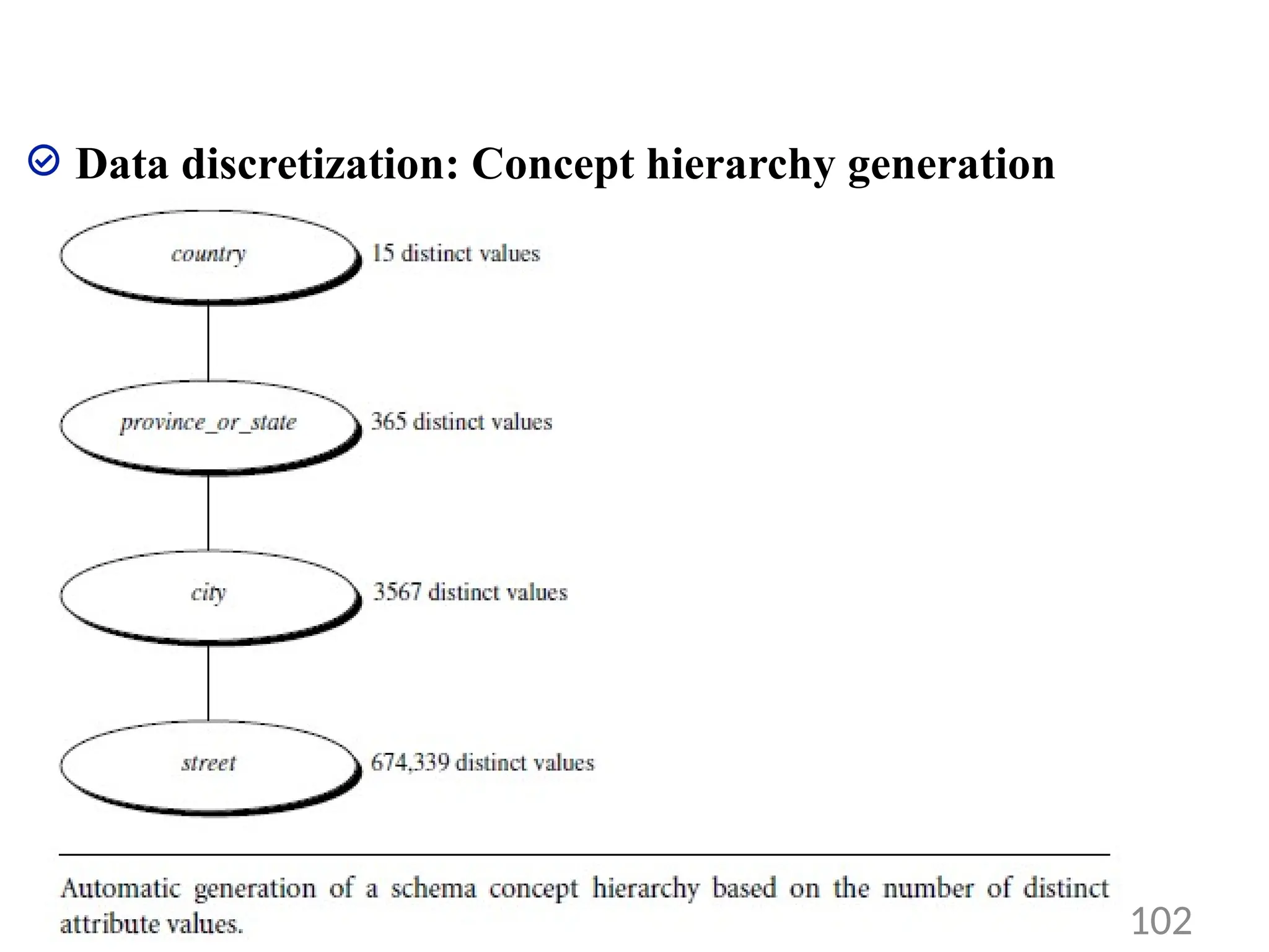
Data discretization: Concepthierarchy generation
3. Specification of a set of attributes, but not of their partial ordering
• The system automatically generate the attribute ordering so as to
construct a meaningful concept hierarchy.
• a concept hierarchy can be automatically generated based on the
number of distinct values per attribute in the given attribute set.
• The attribute with the most distinct values is placed at the lowest
hierarchy level.
• The lower the number of distinct values an attribute has, the higher
it is in the generated concept hierarchy.
• E.g. see the diagram on next slide
101
Data discretization: Concepthierarchy generation
4. Specification of only a partial set of attributes
• Sometimes a user only have a vague idea about what should be
included in a hierarchy.
• Consequently, the user may have included only a small subset of the
relevant attributes in the hierarchy specification
103