IV STATISTICS I.pdf

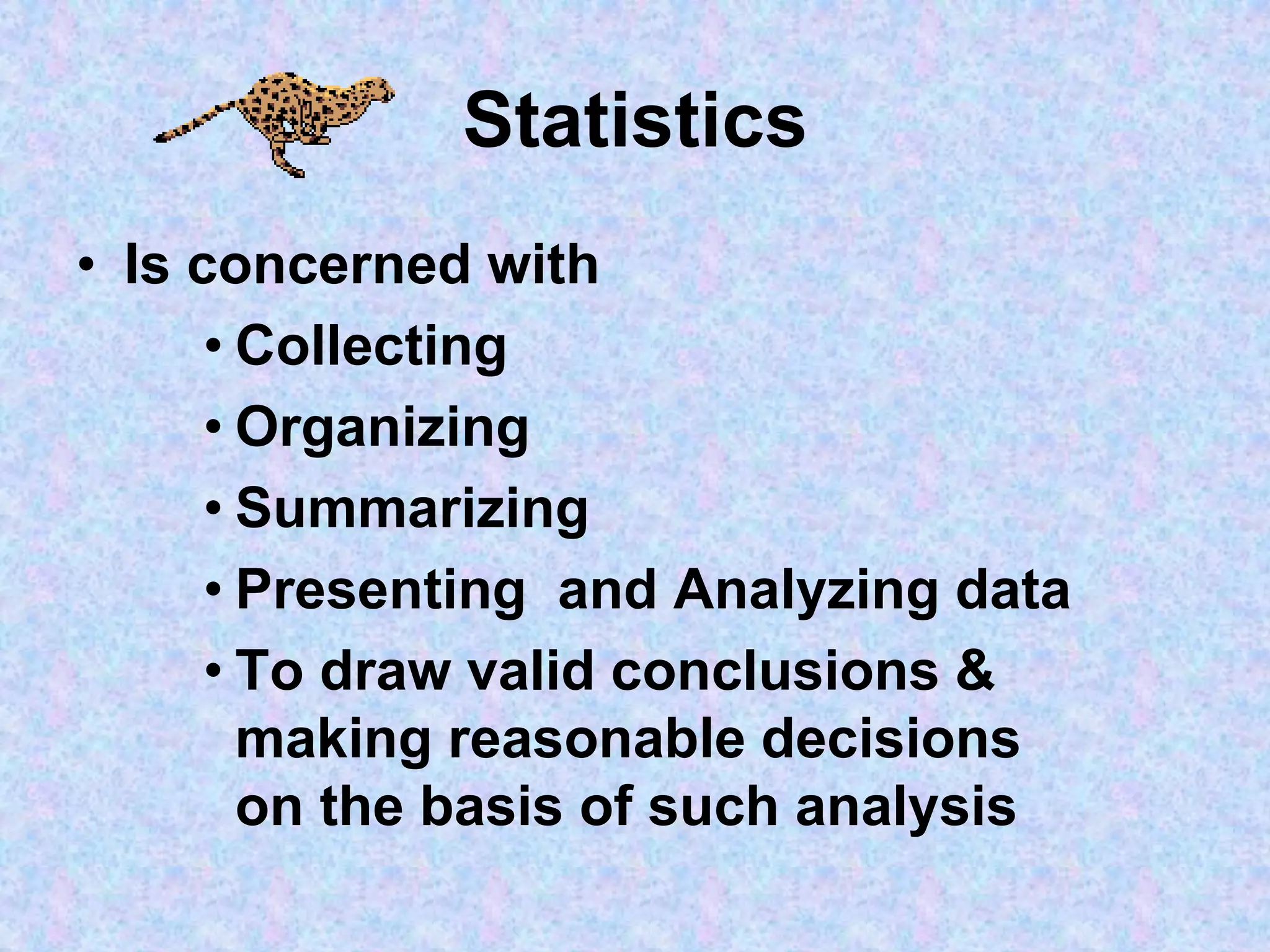
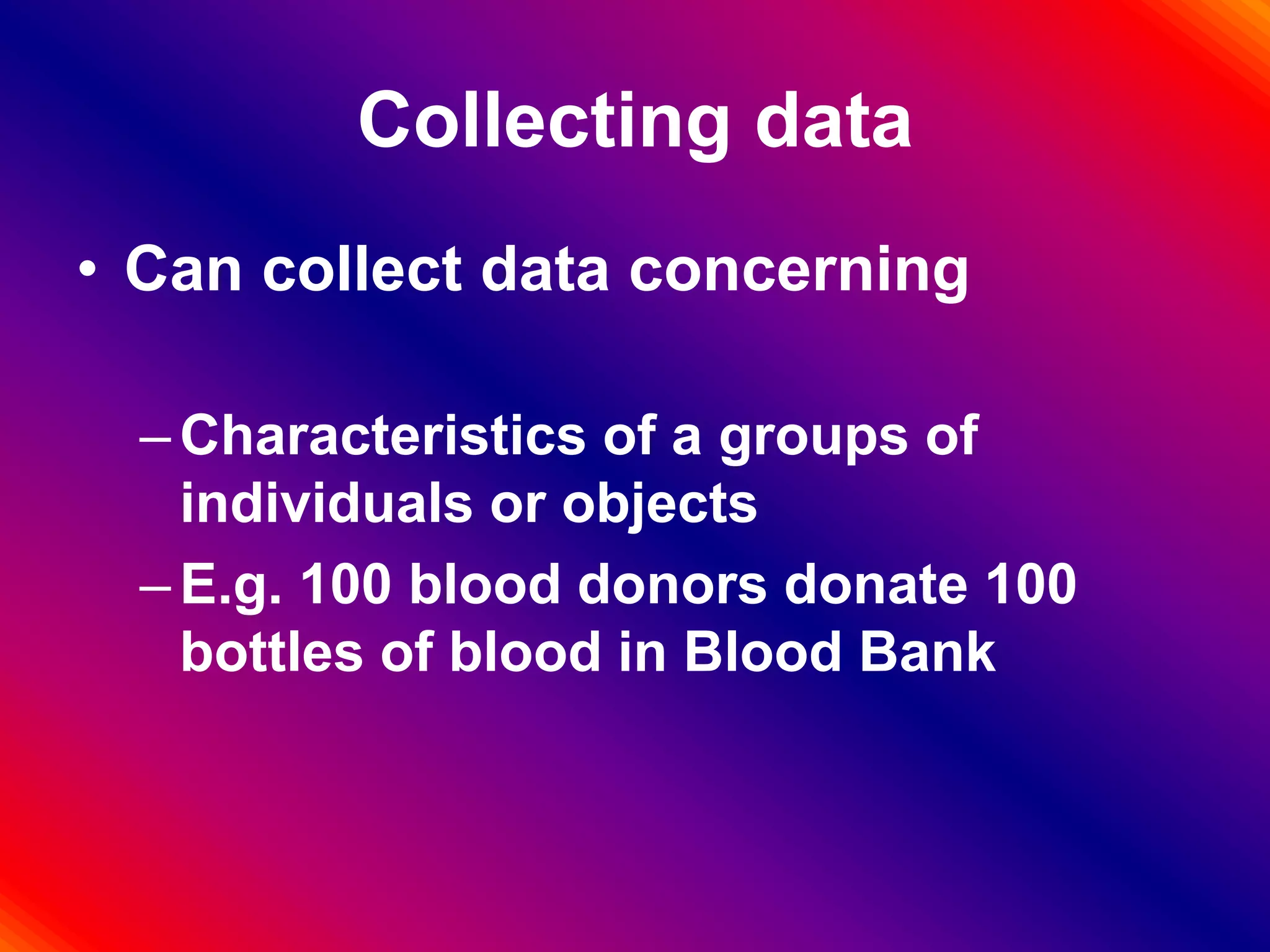
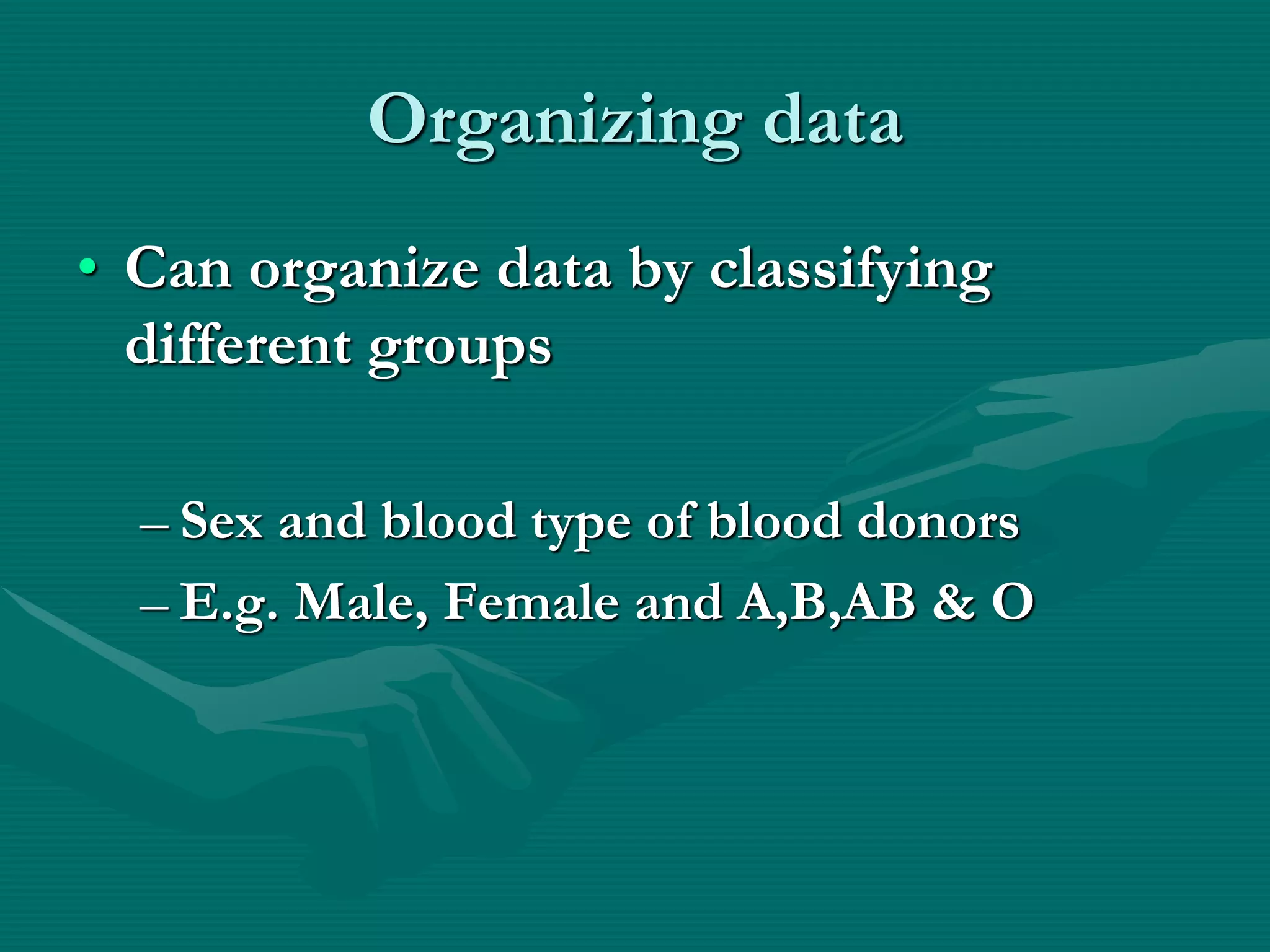
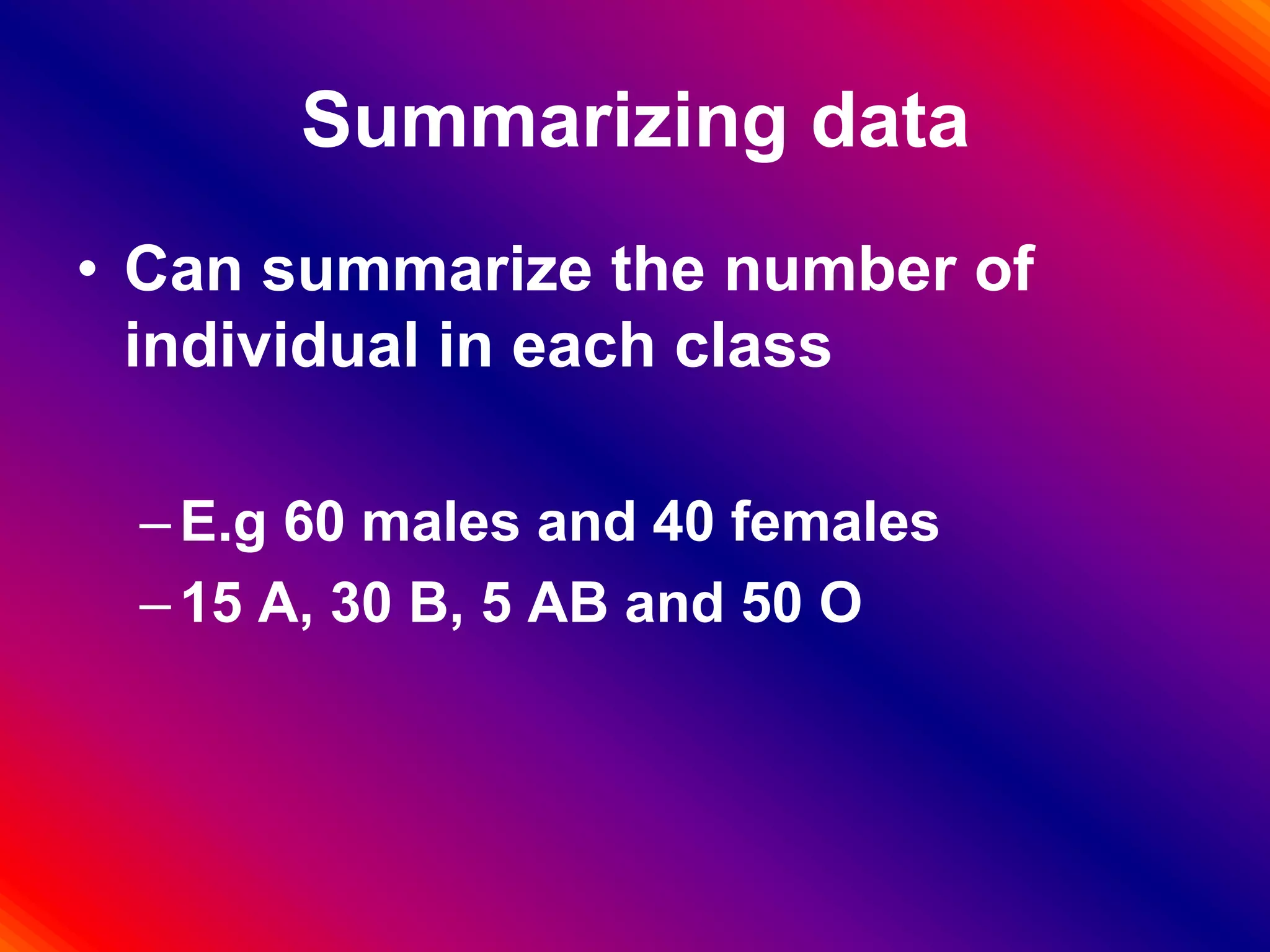
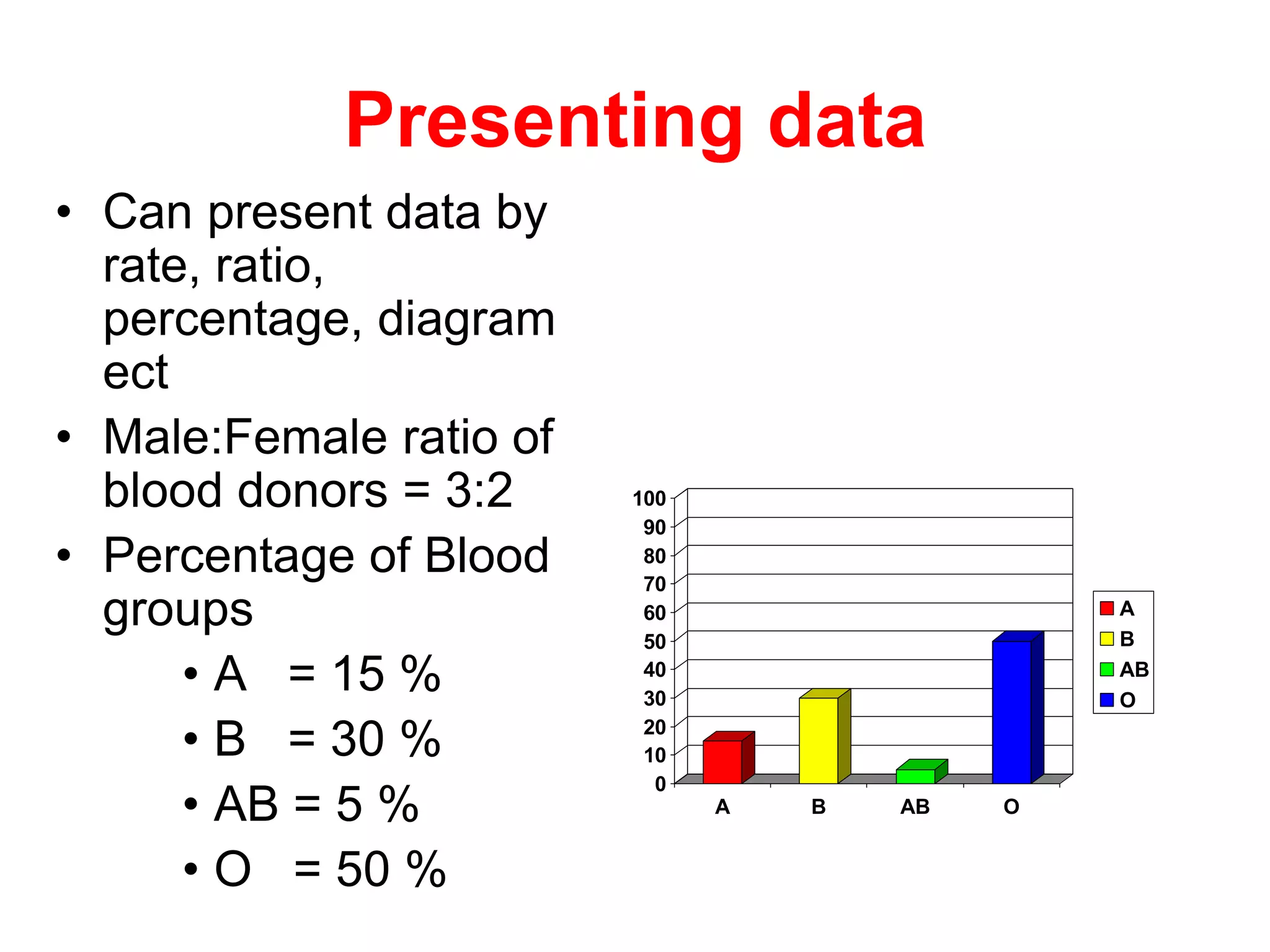
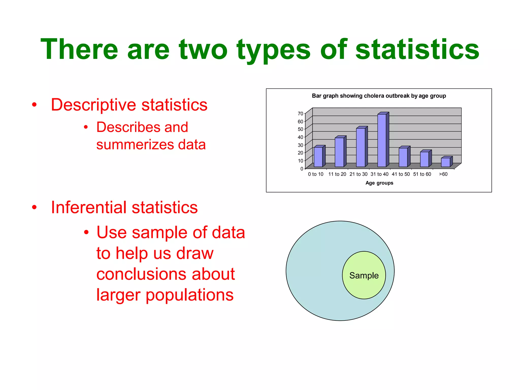
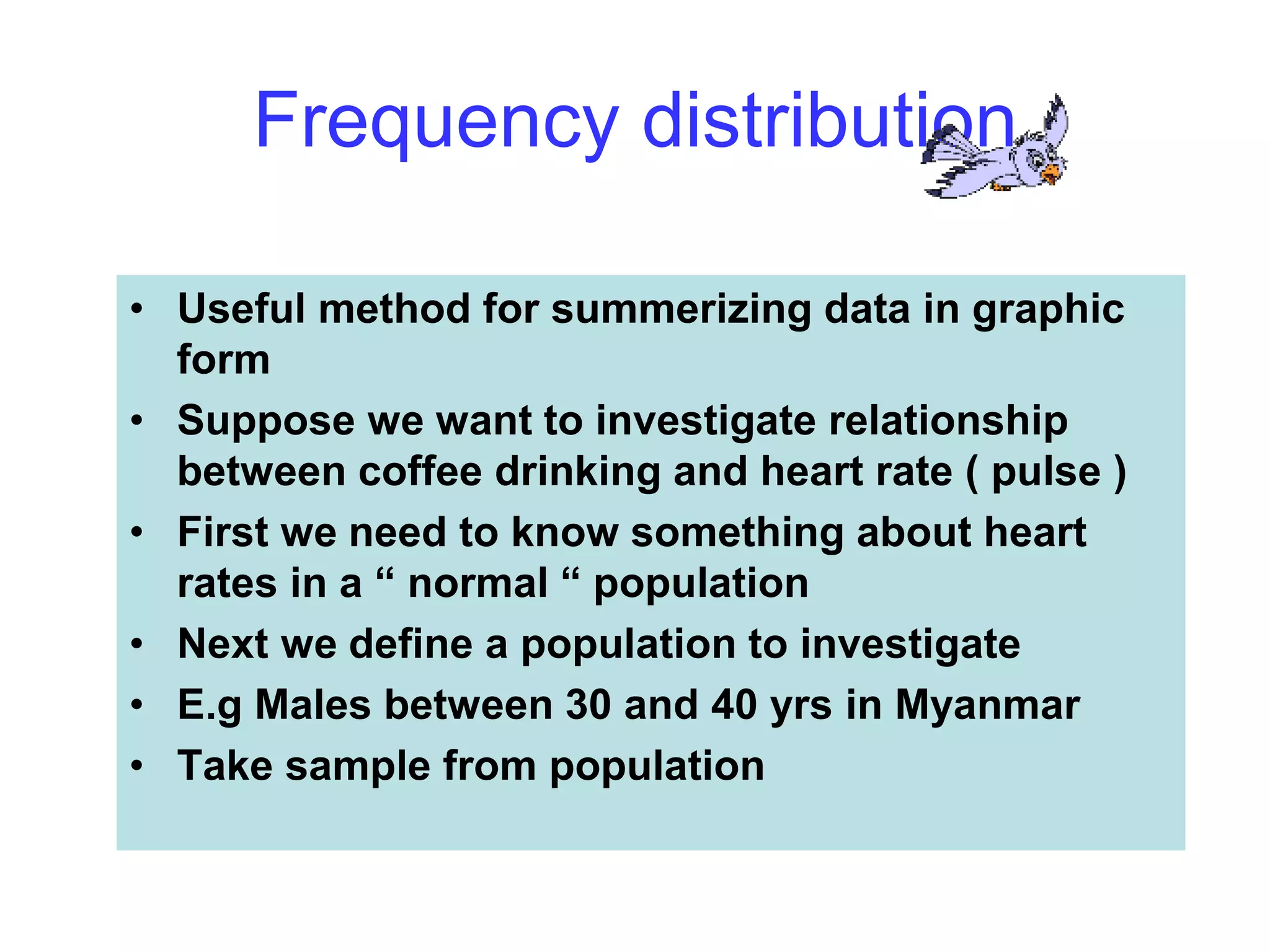
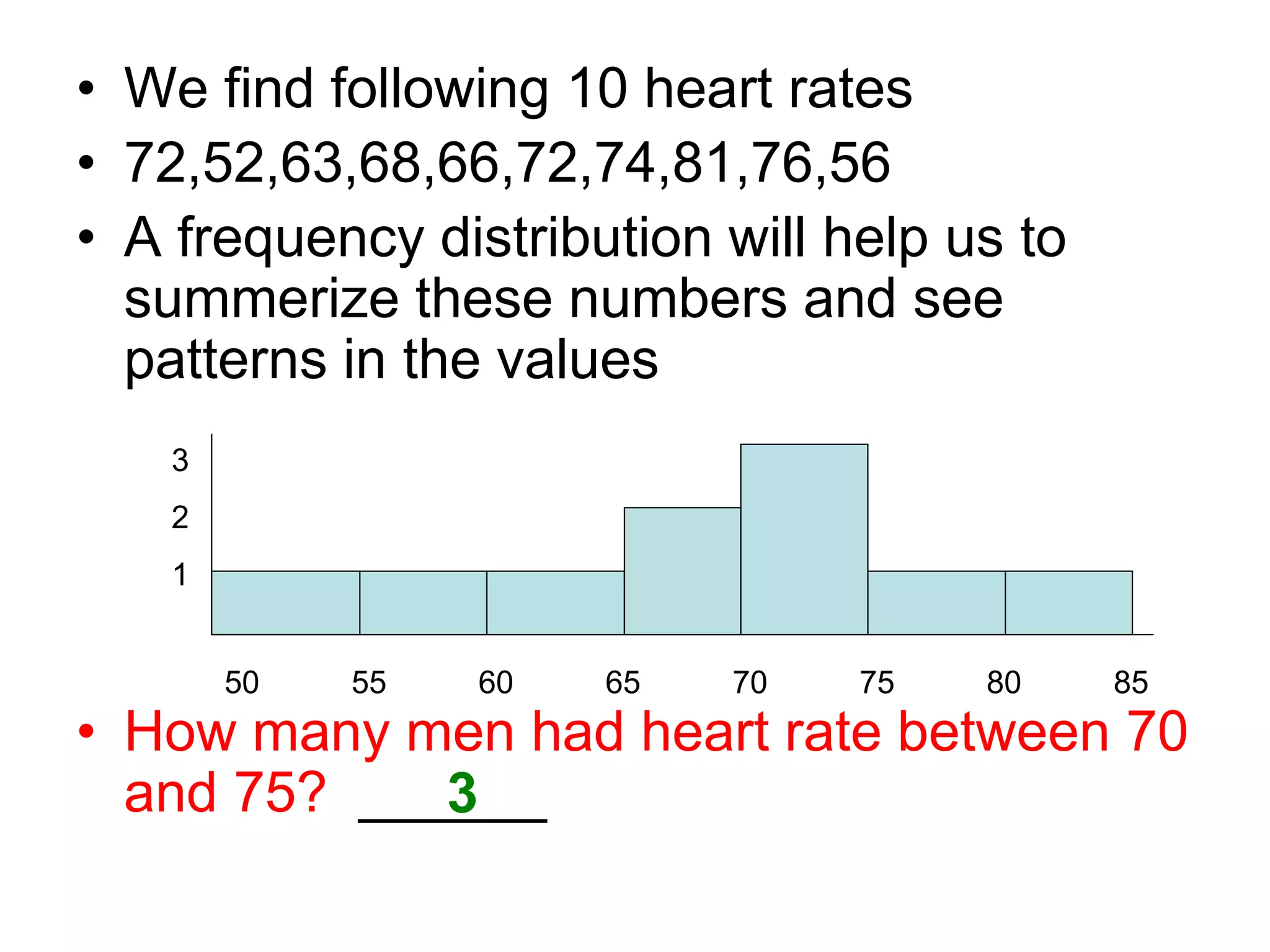
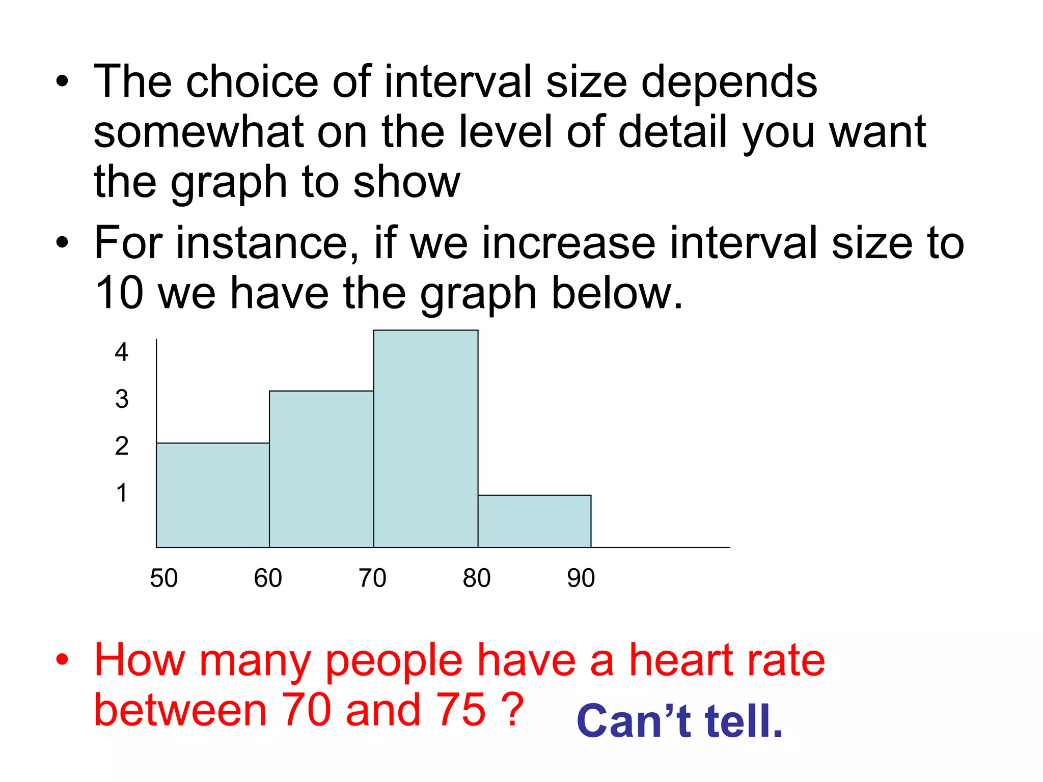
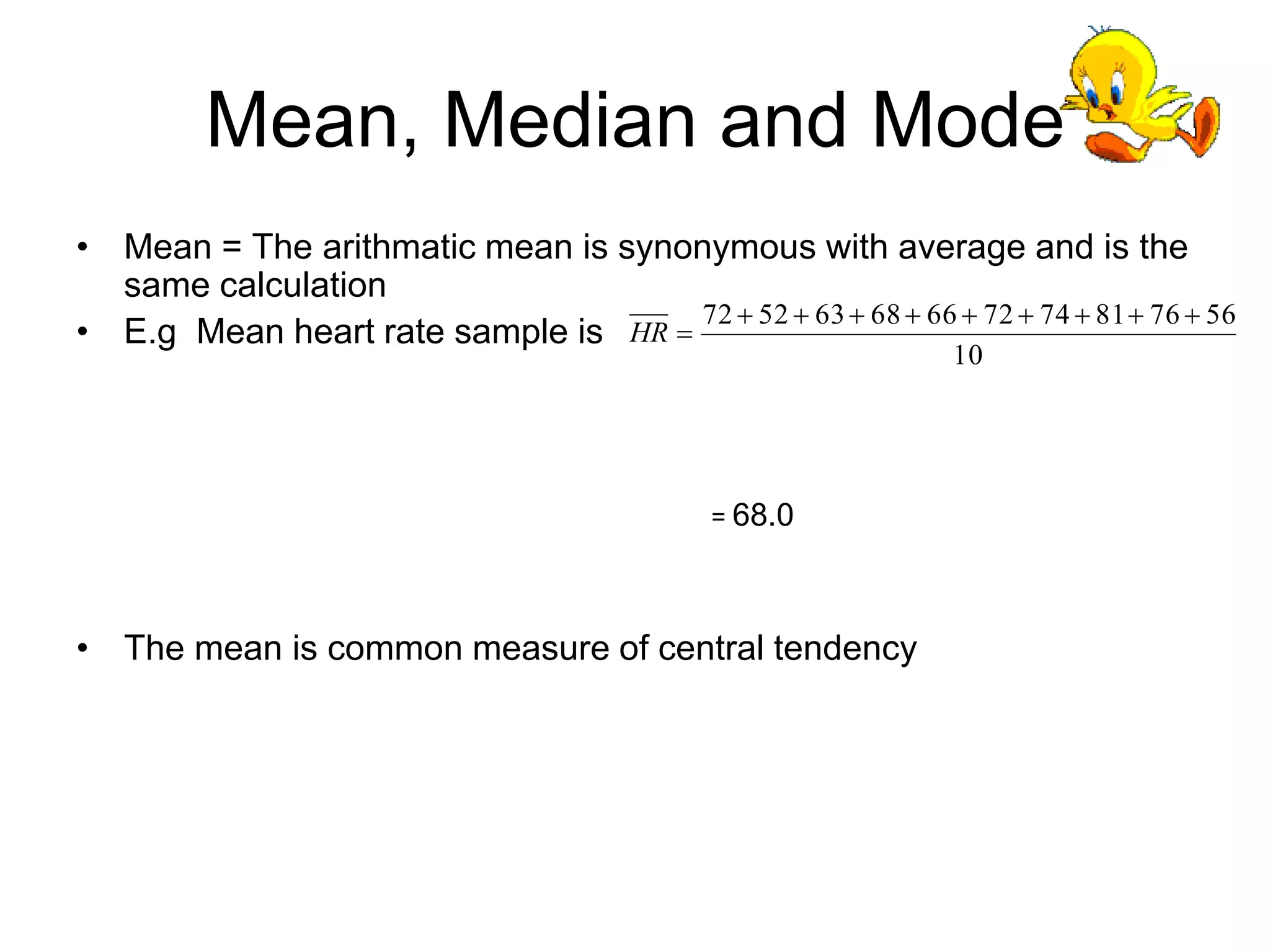
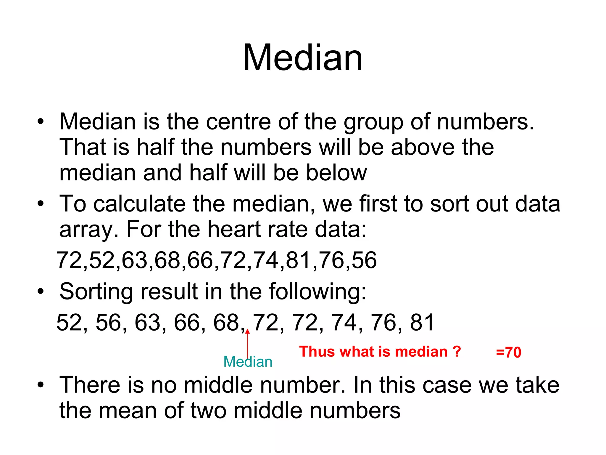
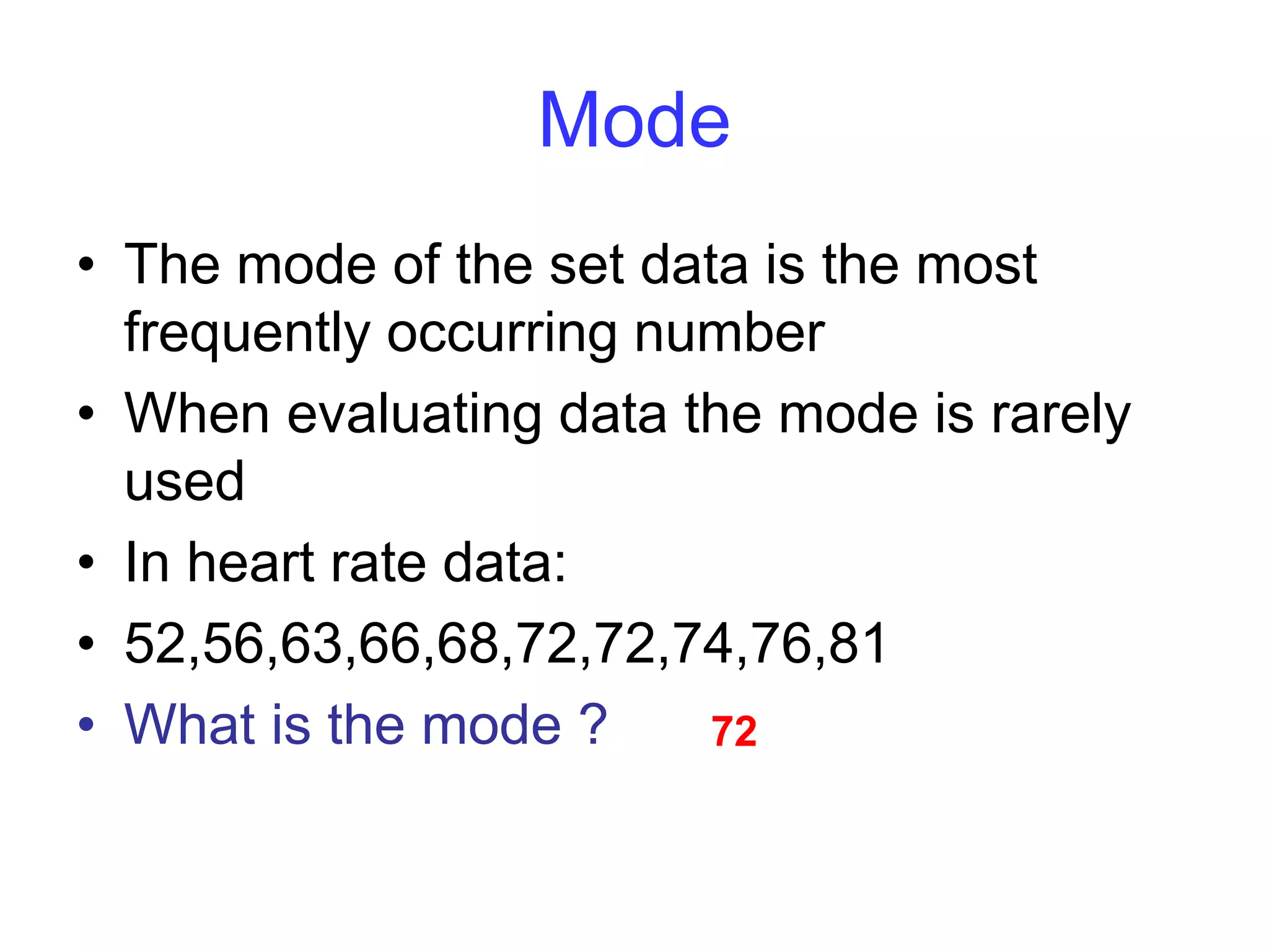
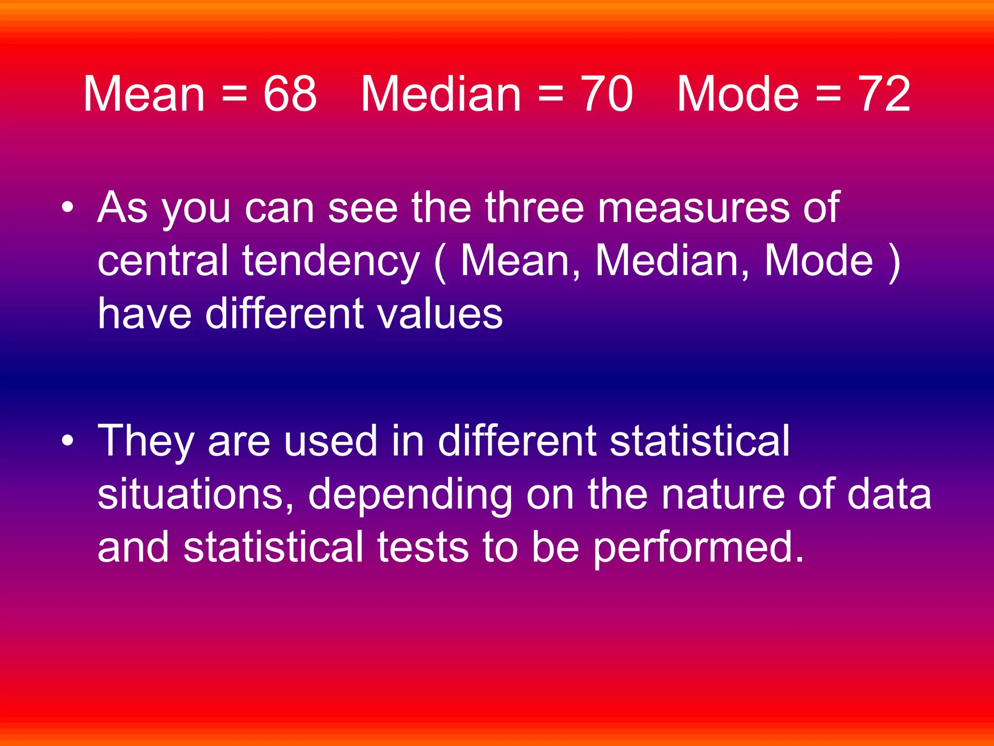
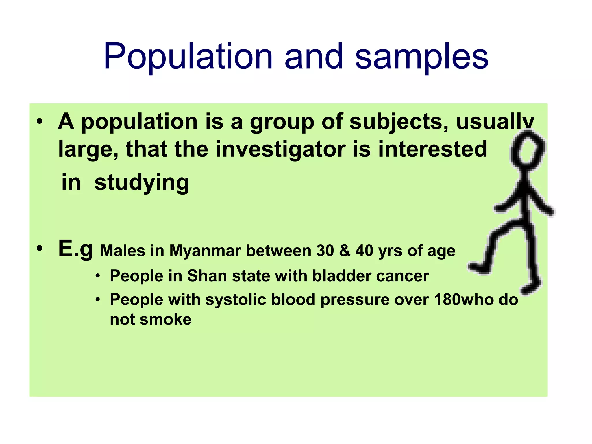
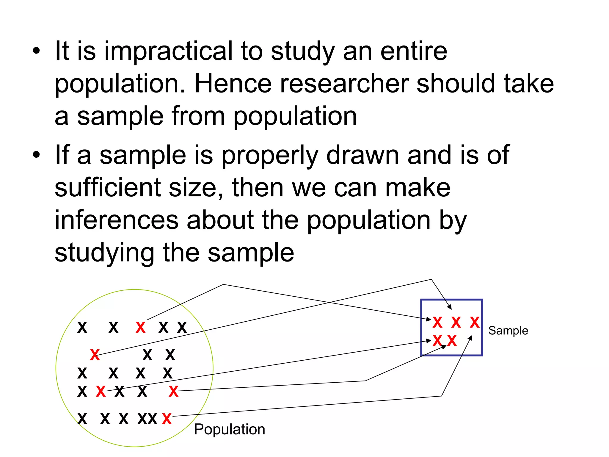
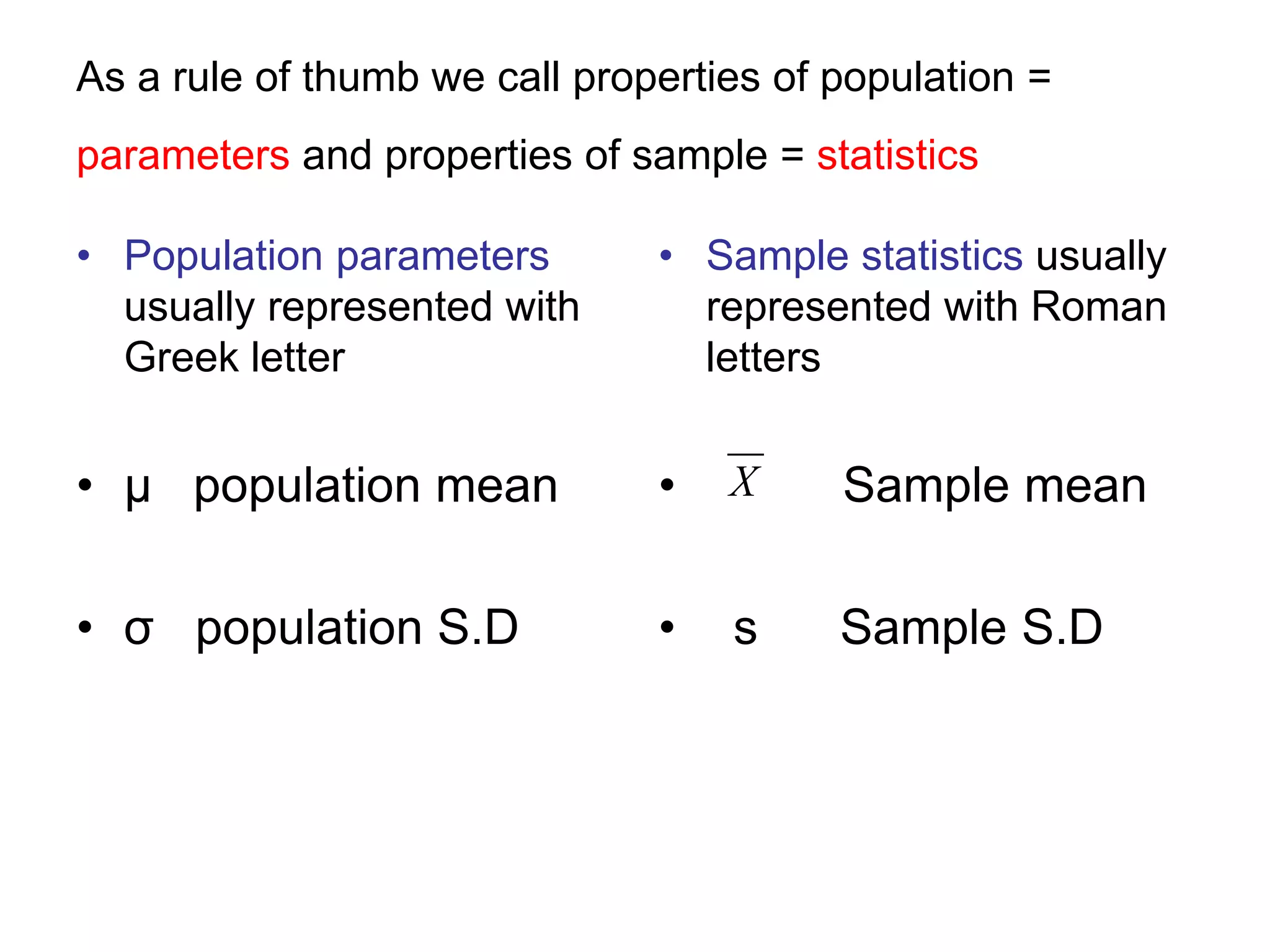
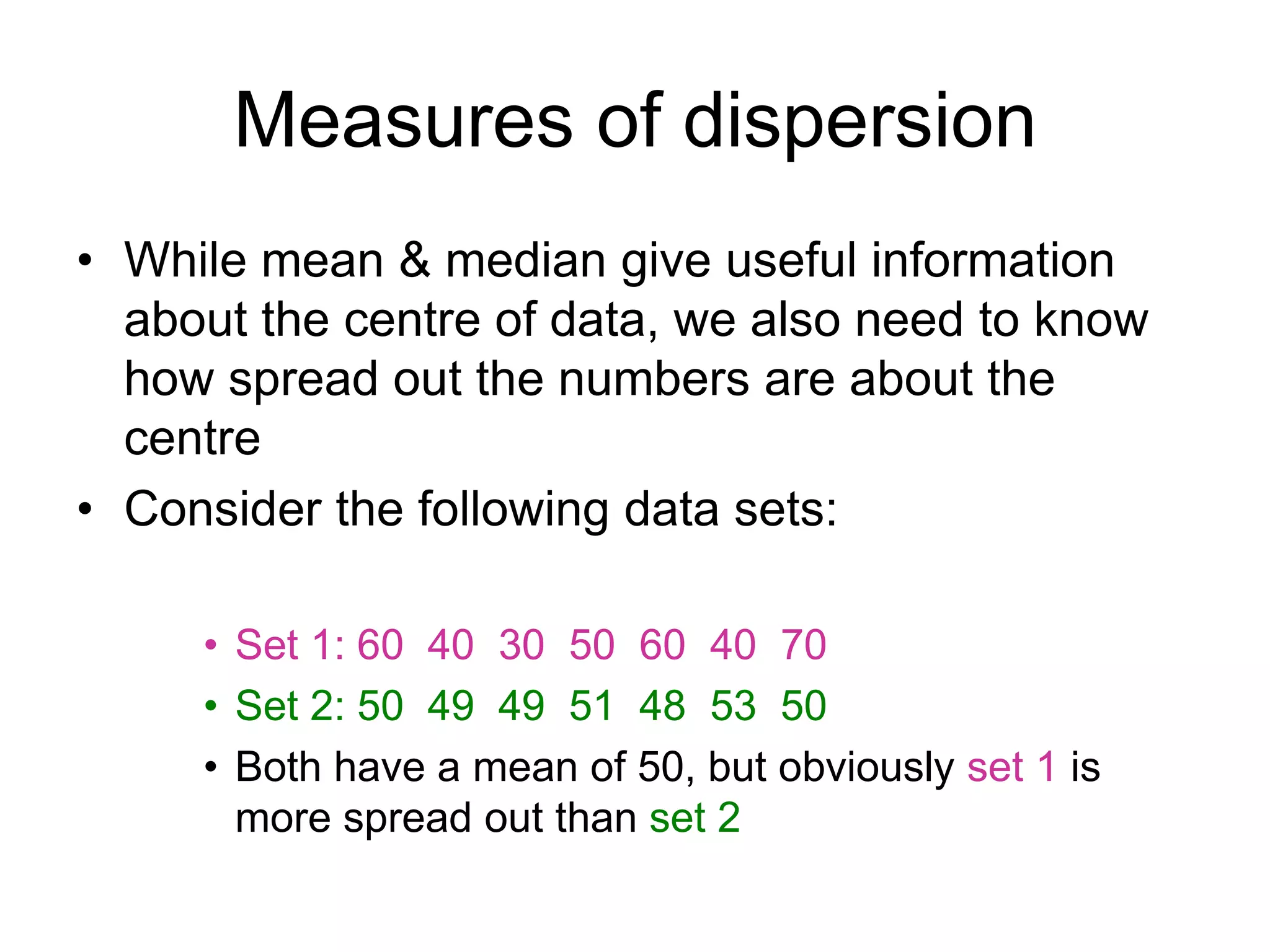
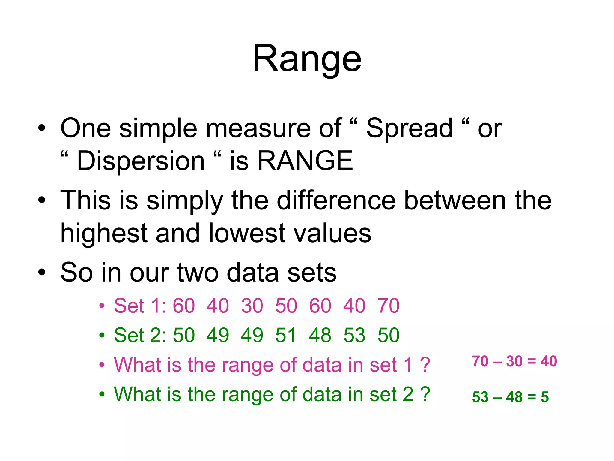
Statistics
• Is concerned with
• Collecting
• Organizing
• Summarizing
• Presenting and Analyzing data
• To draw valid conclusions &
making reasonable decisions
on the basis of such analysis

Collecting data
• Can collect data concerning
–Characteristics of a groups of
individuals or objects
–E.g. 100 blood donors donate 100
bottles of blood in Blood Bank

Organizing data
• Can organize data by classifying
different groups
– Sex and blood type of blood donors
– E.g. Male, Female and A,B,AB & O

Summarizing data
• Can summarize the number of
individual in each class
–E.g 60 males and 40 females
–15 A, 30 B, 5 AB and 50 O

Presenting data
• Can present data by
rate, ratio,
percentage, diagram
ect
• Male:Female ratio of
blood donors = 3:2
• Percentage of Blood
groups
• A = 15 %
• B = 30 %
• AB = 5 %
• O = 50 %
0
10
20
30
40
50
60
70
80
90
100
A B AB O
A
B
AB
O

Analyzing data
• From presentation, the findings can be
analyzed such as more male blood
donors than female

There are two types of statistics
• Descriptive statistics
• Describes and
summerizes data
• Inferential statistics
• Use sample of data
to help us draw
conclusions about
larger populations
0
10
20
30
40
50
60
70
0 to 10 11 to 20 21 to 30 31 to 40 41 to 50 51 to 60 >60
Age groups
Bar graph showing cholera outbreak by age group
Sample

Clinical trial for Antihypertensive drug
• Population with SBP = 180 mm Hg
• Random sample = 10 patients
• Give antihypertensive drug
• After drug, sample mean SBP = 170 mm Hg
• Can we conclude that the drug was effective not
without a statistical analysis?
• No (need to compute probability due to chance )

Descriptive statistics
• Help organize data in more meaningful
way
• Summerize data
• Investigate relationship between variables
• Serve as preliminary analysis before using
inferential technique
• But analysis techniques depend on types
of data

Types of data
• Nominal data
• Ordinal data
• Interval data
• Ratio data

Nominal data
• Refers to data that represent categories or
names
• There is no implied order to the categories
of nominal data
• E.g. Eye colour
• Race
• Gender
• Marital status

Ordinal data
• Refers to data that are ordered but the
space or intervals between data values
are not necessarily equal.
• E.g. Strongly agree
• Agree
• No opinion
• Disagree
• Strongly disagree

Interval data
• Refers the data the interval betweenvalues
are the same
• E.g. Fahrenheit temperature scale
• The difference between 70 degrees and
71 degrees is the same as the difference
between 32 and 33 degrees
• But the scale is not a Ratio scale because
40 degrees F is not twice as much as 20
degrees F ( There is no absolute zero )

Ratio data
• Ratio data do have meaningful ratios e.g.
Age is ratio data.
• Someone who is 40 yrs of age is twice as
old as someone who is 20 yrs
• Temperature Kelvin scale is ratio data
• Most data analysis techniques that apply
Ratio data also apply to interval data

Identify the type of data represented by
each of the following:
• Weight ( Kg )
• Temperature ( Celcius)
• Hair colour
• Job satisfaction index ( 1-5 )
• No. of Heart attack
• Calendar year
• R
• I
• N
• O
• R
• I

Frequency distribution
• Useful method for summerizing data in graphic
form
• Suppose we want to investigate relationship
between coffee drinking and heart rate ( pulse )
• First we need to know something about heart
rates in a “ normal “ population
• Next we define a population to investigate
• E.g Males between 30 and 40 yrs in Myanmar
• Take sample from population

• We find following 10 heart rates
• 72,52,63,68,66,72,74,81,76,56
• A frequency distribution will help us to
summerize these numbers and see
patterns in the values
• How many men had heart rate between 70
and 75? ______
50 55 60 65 70 75 80 85
3
2
1
3

• The choice of interval size depends
somewhat on the level of detail you want
the graph to show
• For instance, if we increase interval size to
10 we have the graph below.
• How many people have a heart rate
between 70 and 75 ?
50 60 70 80 90
4
3
2
1
Can’t tell.

Mean, Median and Mode
• Mean = The arithmatic mean is synonymous with average and is the
same calculation
• E.g Mean heart rate sample is
= 68.0
• The mean is common measure of central tendency
10
56
76
81
74
72
66
68
63
52
72 









HR

Median
• Median is the centre of the group of numbers.
That is half the numbers will be above the
median and half will be below
• To calculate the median, we first to sort out data
array. For the heart rate data:
72,52,63,68,66,72,74,81,76,56
• Sorting result in the following:
52, 56, 63, 66, 68, 72, 72, 74, 76, 81
• There is no middle number. In this case we take
the mean of two middle numbers
Median
Thus what is median ? =70

Mode
• The mode of the set data is the most
frequently occurring number
• When evaluating data the mode is rarely
used
• In heart rate data:
• 52,56,63,66,68,72,72,74,76,81
• What is the mode ? 72

Mean = 68 Median = 70 Mode = 72
• As you can see the three measures of
central tendency ( Mean, Median, Mode )
have different values
• They are used in different statistical
situations, depending on the nature of data
and statistical tests to be performed.

Population and samples
• A population is a group of subjects, usually
large, that the investigator is interested
in studying
• E.g Males in Myanmar between 30 & 40 yrs of age
• People in Shan state with bladder cancer
• People with systolic blood pressure over 180who do
not smoke

• It is impractical to study an entire
population. Hence researcher should take
a sample from population
• If a sample is properly drawn and is of
sufficient size, then we can make
inferences about the population by
studying the sample
Population
Sample
X X X X X
X X X
X X X X
X X X X X
X X X XX X
X X X
X X

As a rule of thumb we call properties of population =
parameters and properties of sample = statistics
• Population parameters
usually represented with
Greek letter
• μ population mean
• σ population S.D
• Sample statistics usually
represented with Roman
letters
• Sample mean
• s Sample S.D
X

Measures of dispersion
• While mean & median give useful information
about the centre of data, we also need to know
how spread out the numbers are about the
centre
• Consider the following data sets:
• Set 1: 60 40 30 50 60 40 70
• Set 2: 50 49 49 51 48 53 50
• Both have a mean of 50, but obviously set 1 is
more spread out than set 2

Range
• One simple measure of “ Spread “ or
“ Dispersion “ is RANGE
• This is simply the difference between the
highest and lowest values
• So in our two data sets
• Set 1: 60 40 30 50 60 40 70
• Set 2: 50 49 49 51 48 53 50
• What is the range of data in set 1 ?
• What is the range of data in set 2 ?
70 – 30 = 40
53 – 48 = 5

• However you will find that the range is not
often used, and for good reason it is too
sensitive to a single high or low data value
• Instead we suggest two alternatives:
• Inter quartile range
• Standard deviation

Inter quartile range
• The inter quartile range is similar to the range
except that it measures the difference between
the first and third quartiles
• To compute it, we first sort the data.
• Then find the data values correspondingly to the
first quarter of the numbers ( first quartile ) and
then top quarter ( third quartile )
• The inter quartile range is the distance between
these quartiles

• Given the following data set:
18 21 23 24 24 32 42 59
• We sort the data from lowest and highest
• Find the bottom quarter and top quarter of
the data
• Then determine the range between these
values
• What do you get for the inter quartile range ?
First quartile = 22 Third quartile = 37
13

Why is inter quartile range preferable
measure to the range ?
1. It is a smaller number
2. It is less prone to distortion by a single
large or small value
3. It is easier to calculate
– Enter 1, 2, 3
Yes, outliers in the data do not effect the inter quartile
range

Standard deviation
• The most common used measure of
dispersion is Standard Deviation
• The S.D can be thought of as the “
average “ deviation ( difference ) between
the mean of a sample and each data value
in the sample

• The actual formula squares all the deviations to
make them all positive and takes the square
root at the end
• Where = sample mean = summation operation
• = individual sample value
• n = number of data points in a sample
1
)
( 2




n
x
x
SD
i
x
i
x

• As an example , let’s compute the standard deviation of
the four values
• 1 3 5 7
• Step 1 – Calculate the mean = Σ x / n = 4
• Step 2 – Compute the deviation of each score from the
mean
Value Mean Deviation Step 3 – Square all
deviations and add
square deviation
1 4 -3 9
3 4 -1 1
5 4 +1 1
7 4 +3 9
20

• Step 4 – Divided by n – 1 = 20 / 3
• Step 5 – Take the square root
Review
• Step 1 – Calculate mean
• Step 2 – Compute deviation
• Step 3 – Square and sum
• Step 4 – Divide by n – 1
• Step 5 – Take square root
• By the way the quantity before we take the square root is called
Variance
• Variance = ( Standard deviation
58
.
2
3
/
20 
2
)
x
x
xi 
  2
)
( x
xi
)
1
/(
)
( 2


 n
x
xi
1
)
( 2



n
x
xi

IV STATISTICS I.pdf

More Related Content

Similar to IV STATISTICS I.pdf

Recently uploaded

IV STATISTICS I.pdf