Download as PDF, PPTX
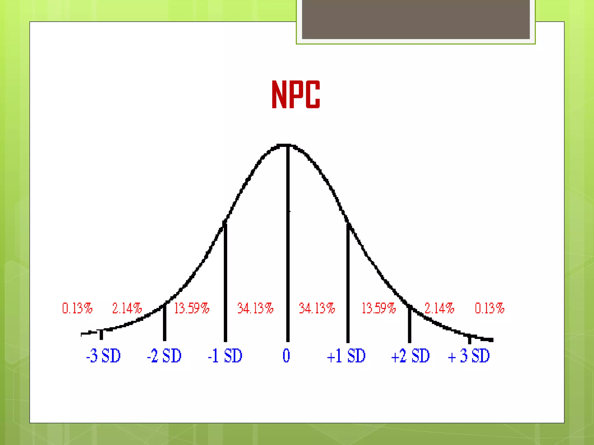


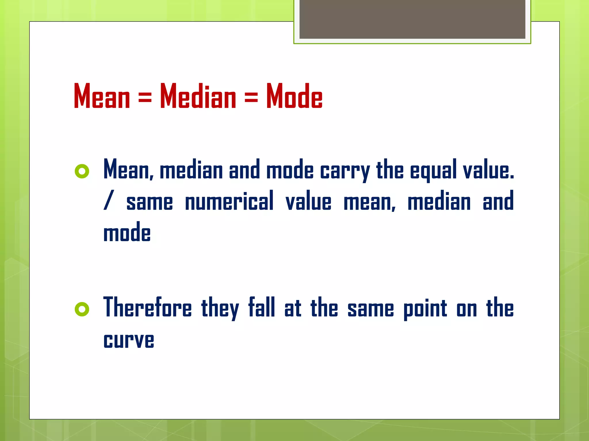

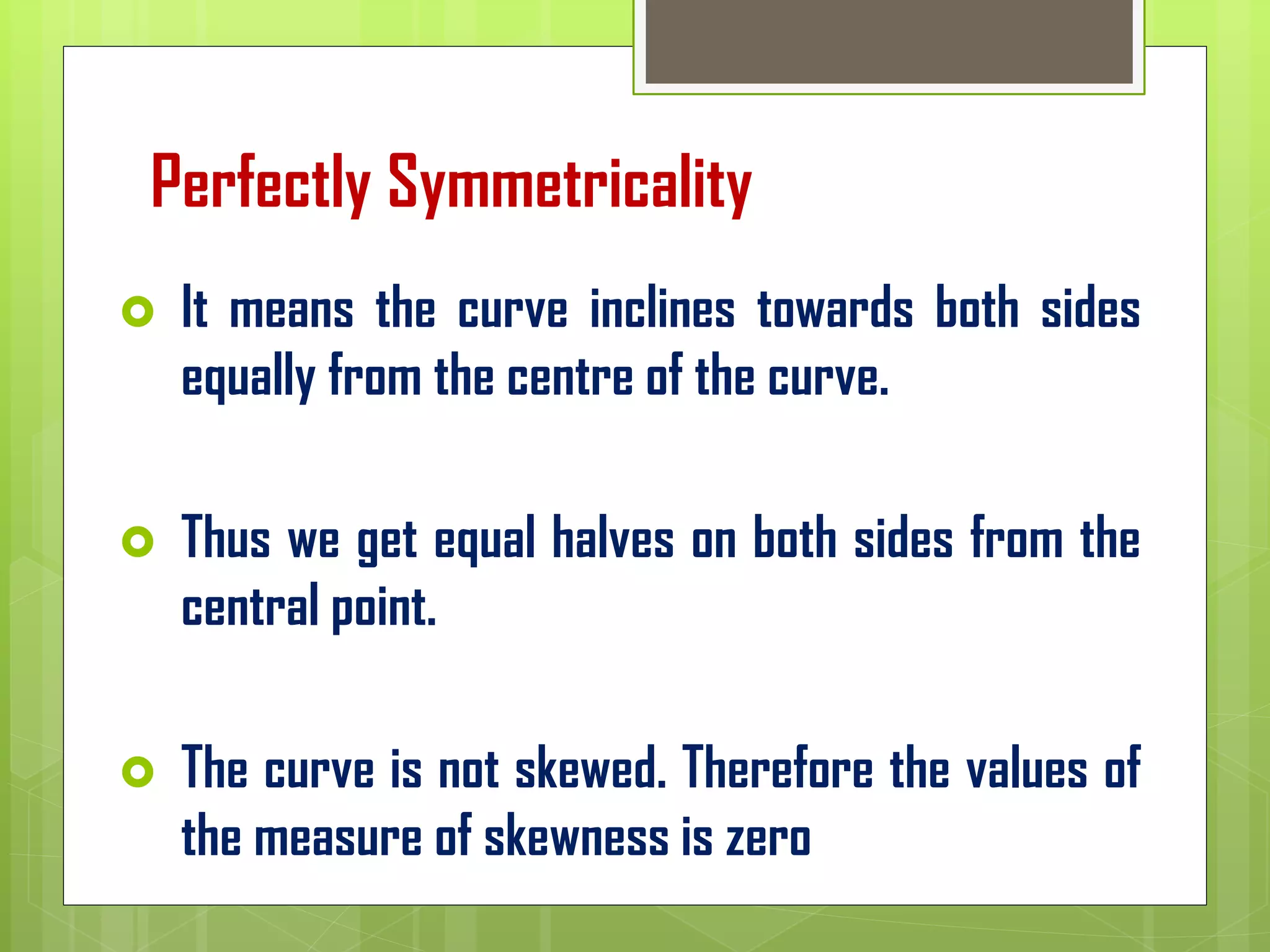
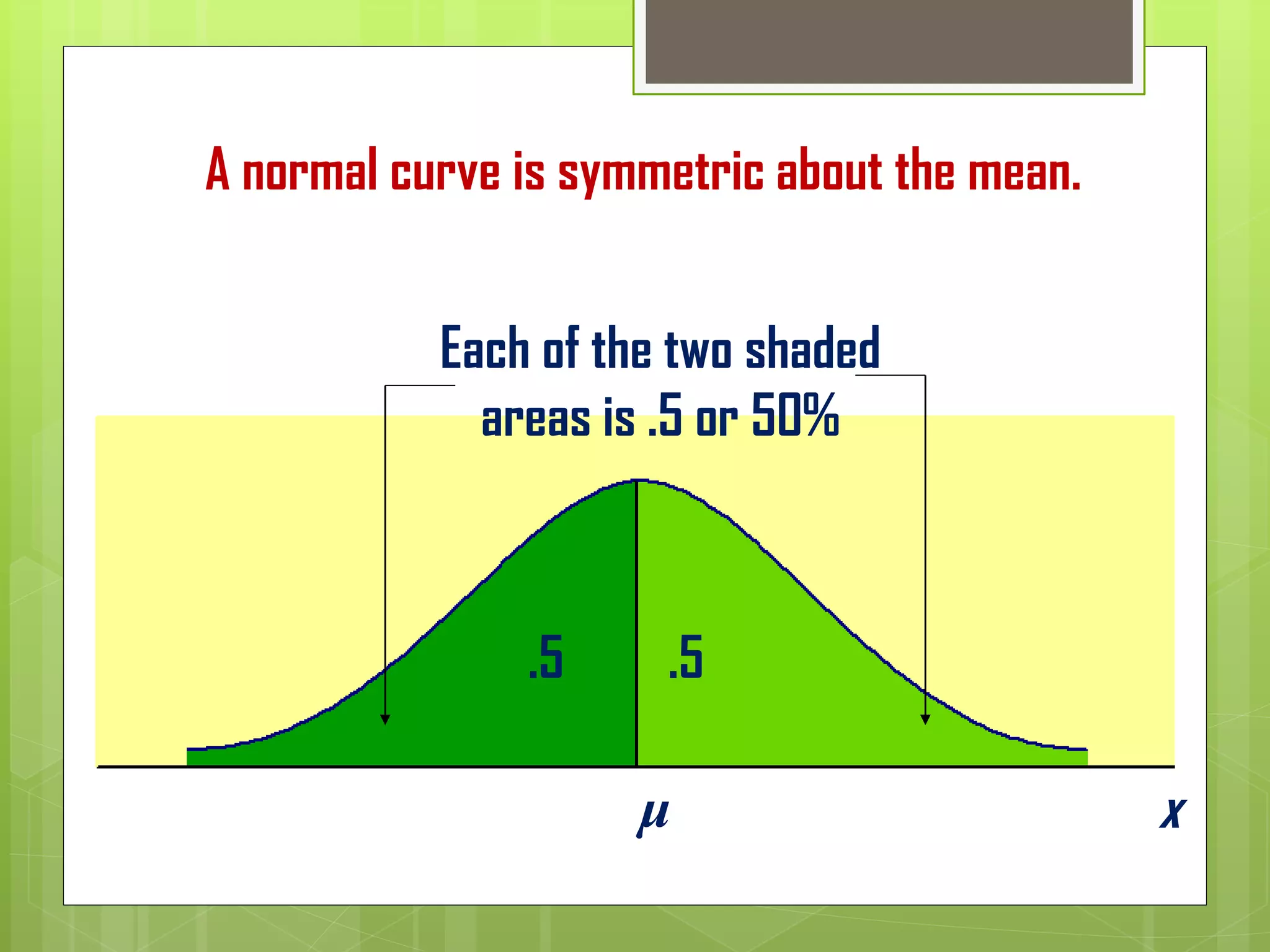
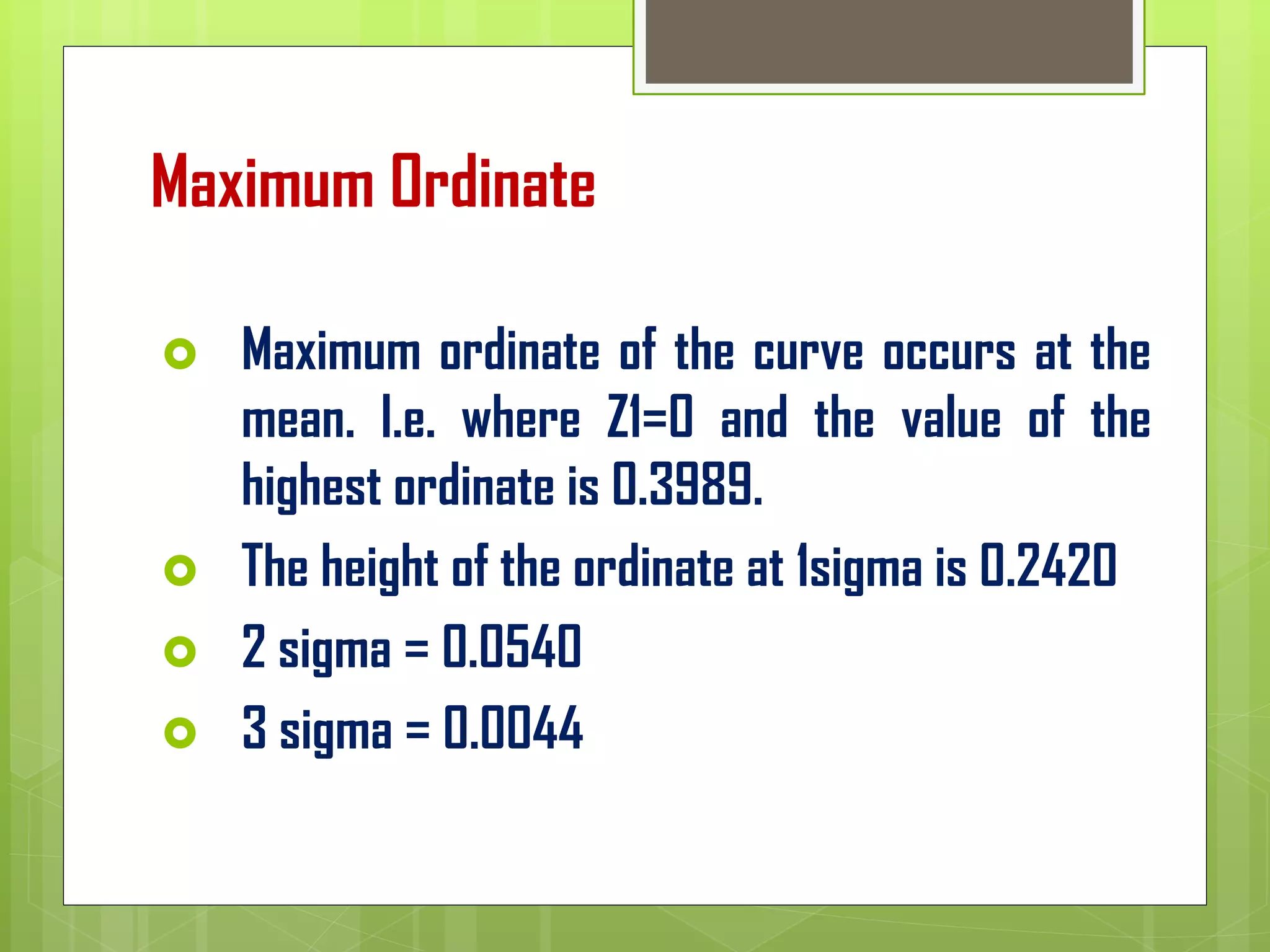
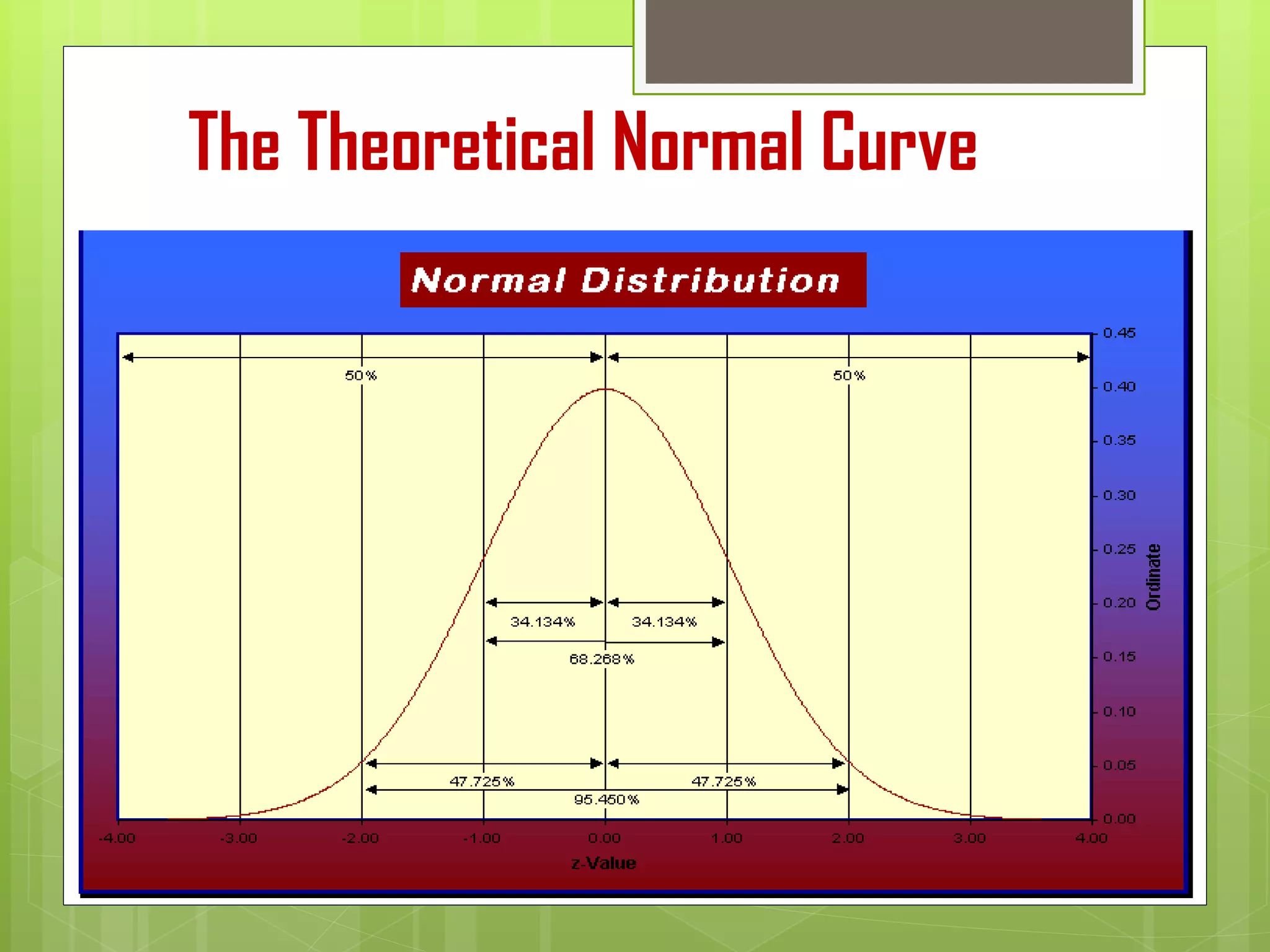
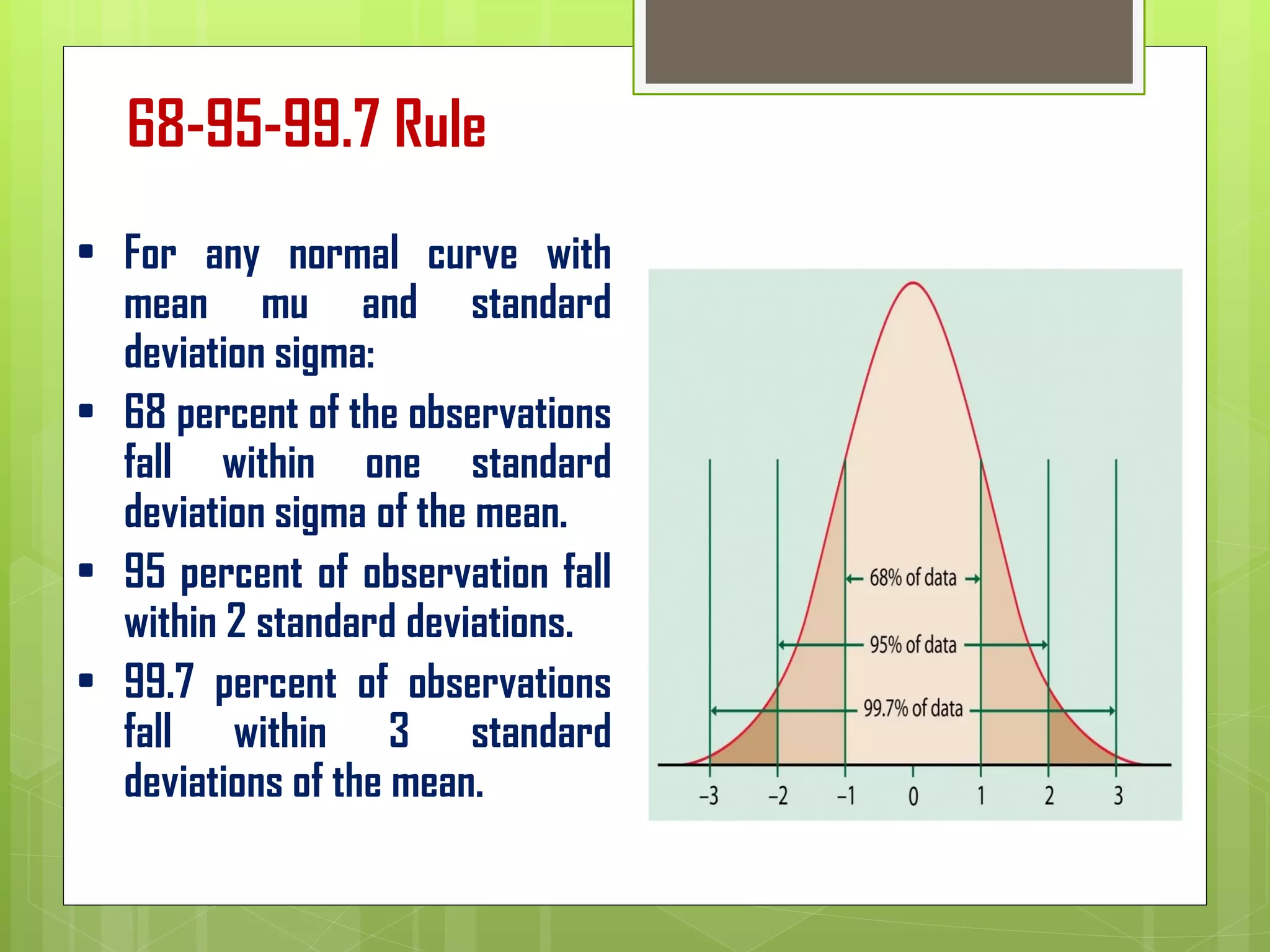
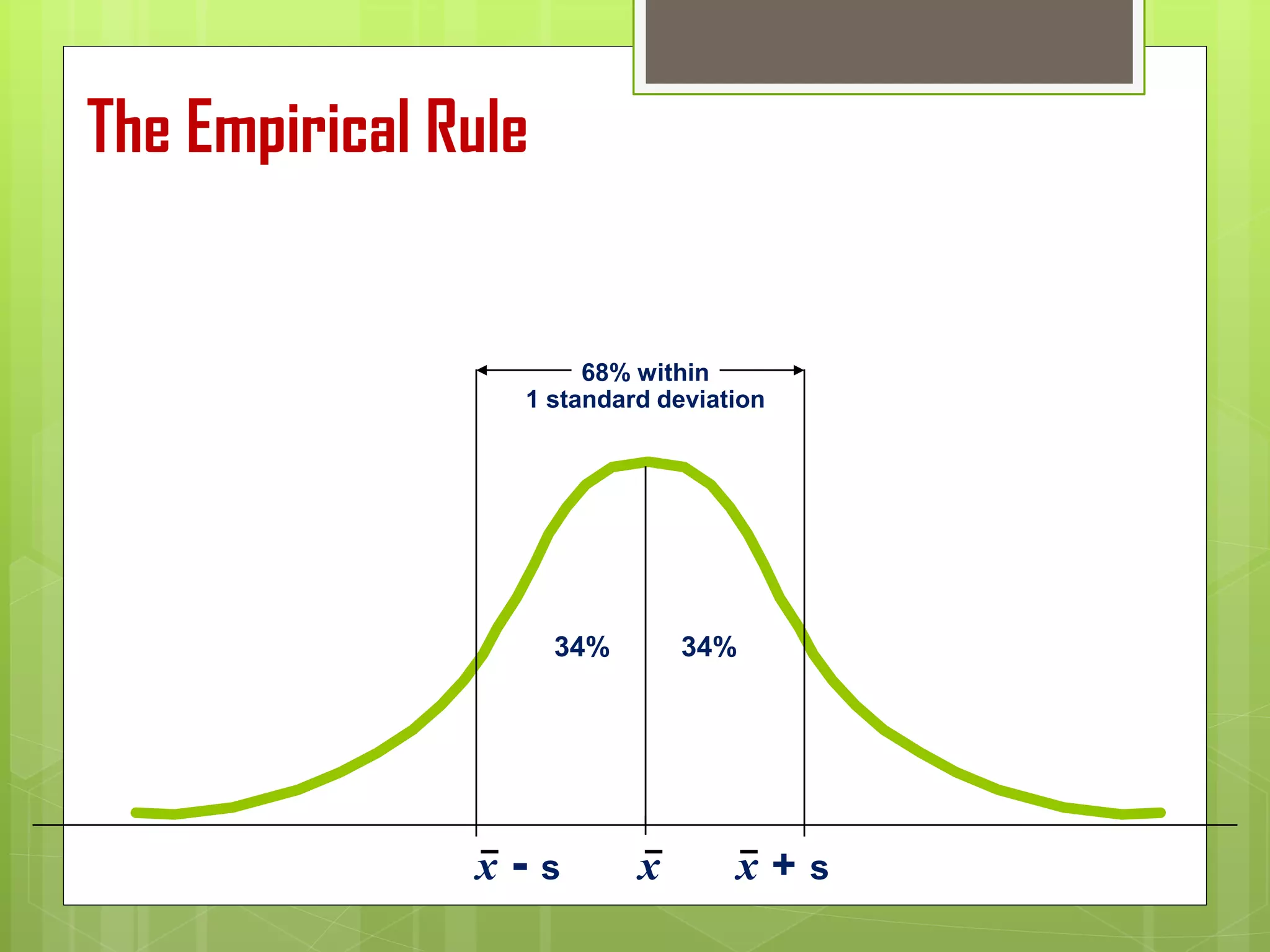
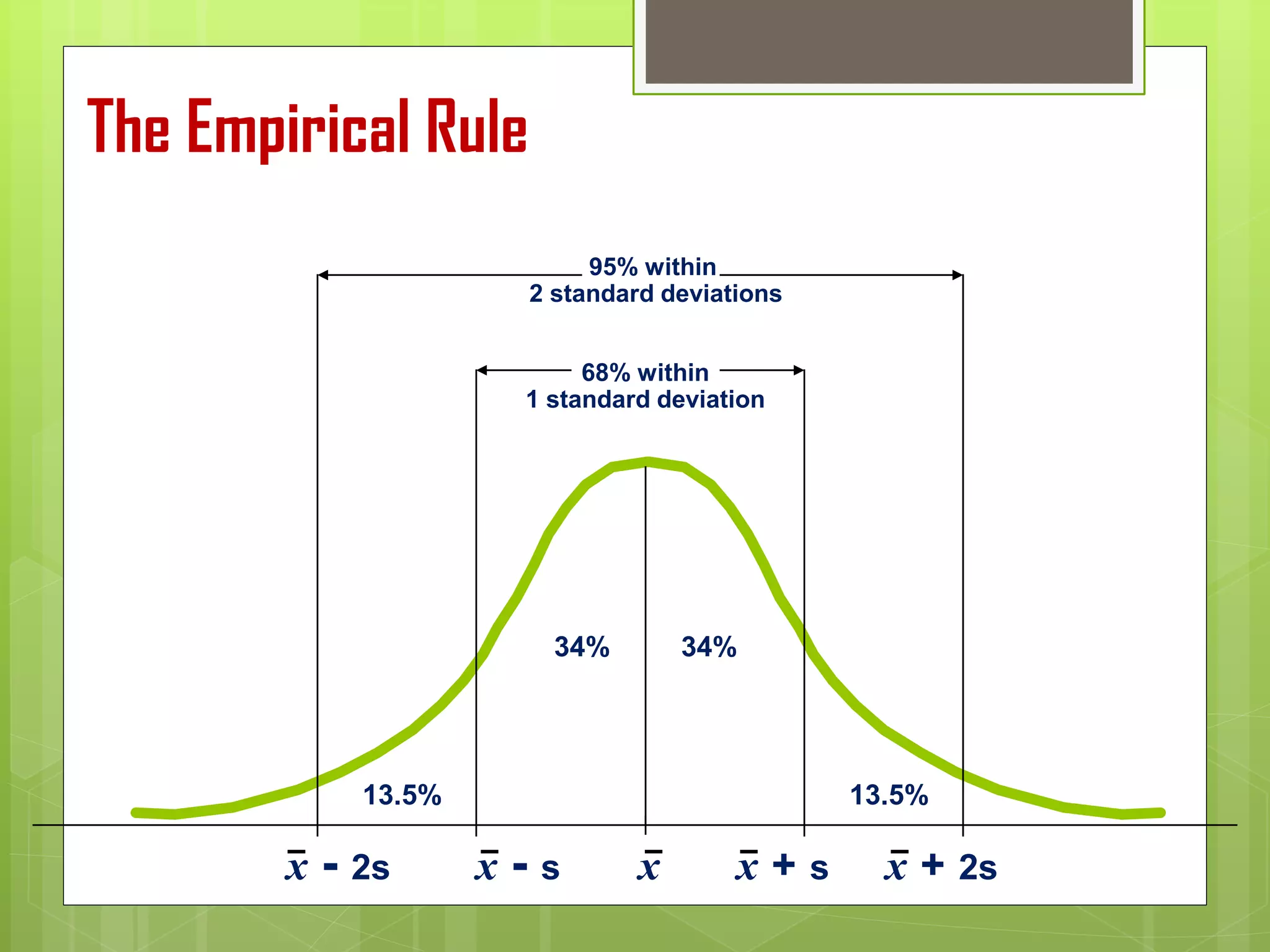
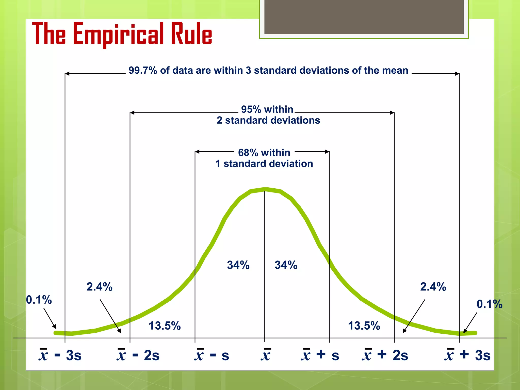
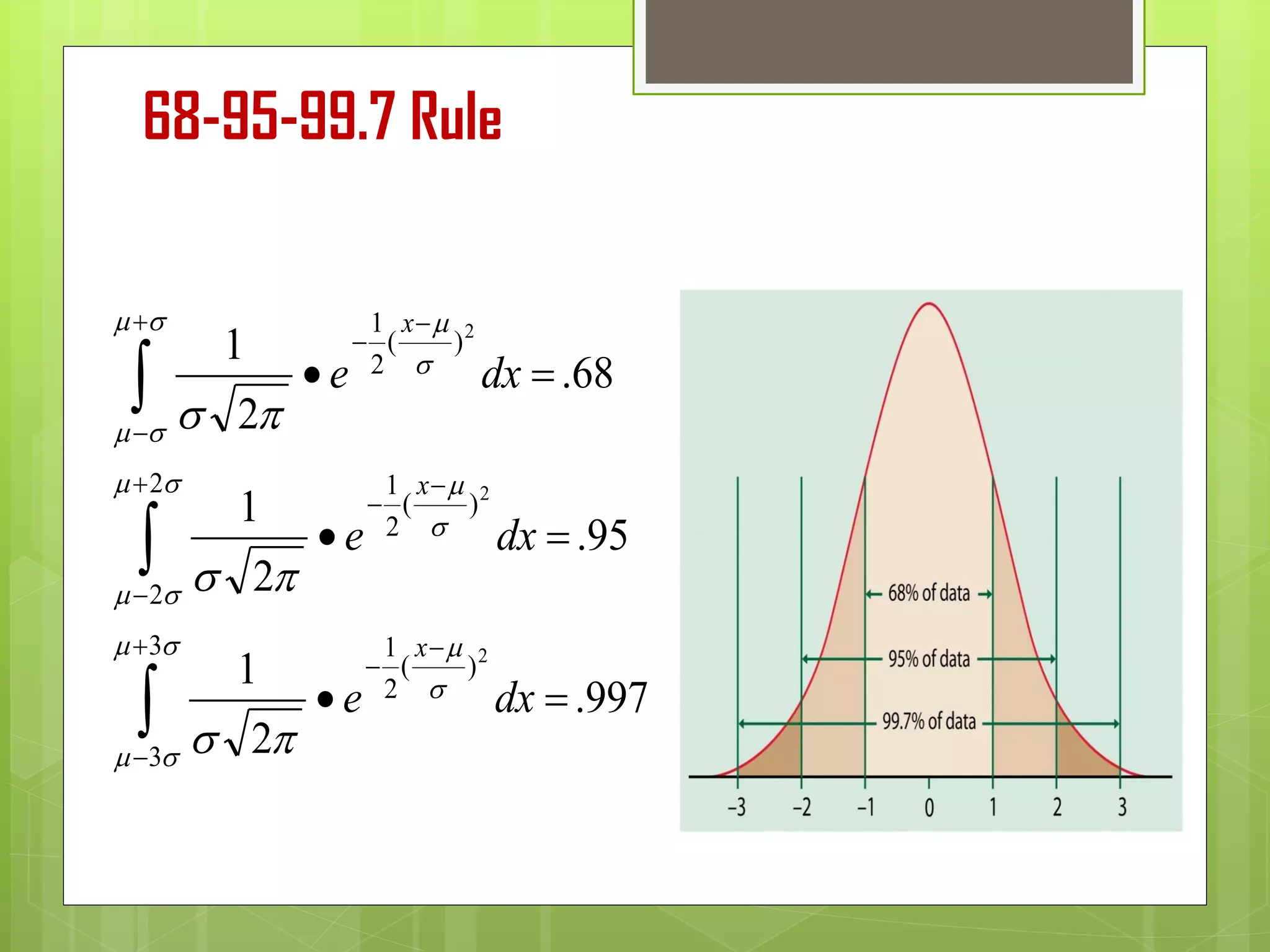
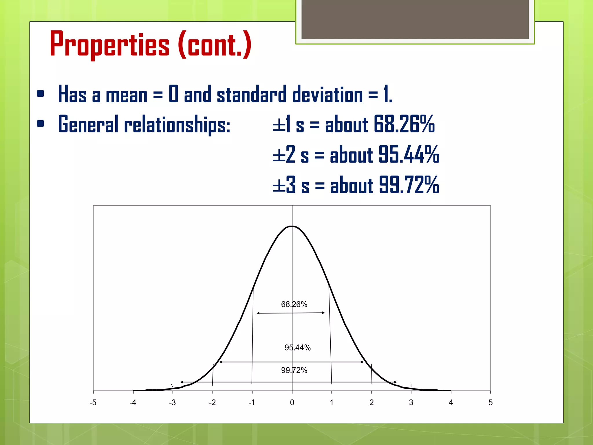


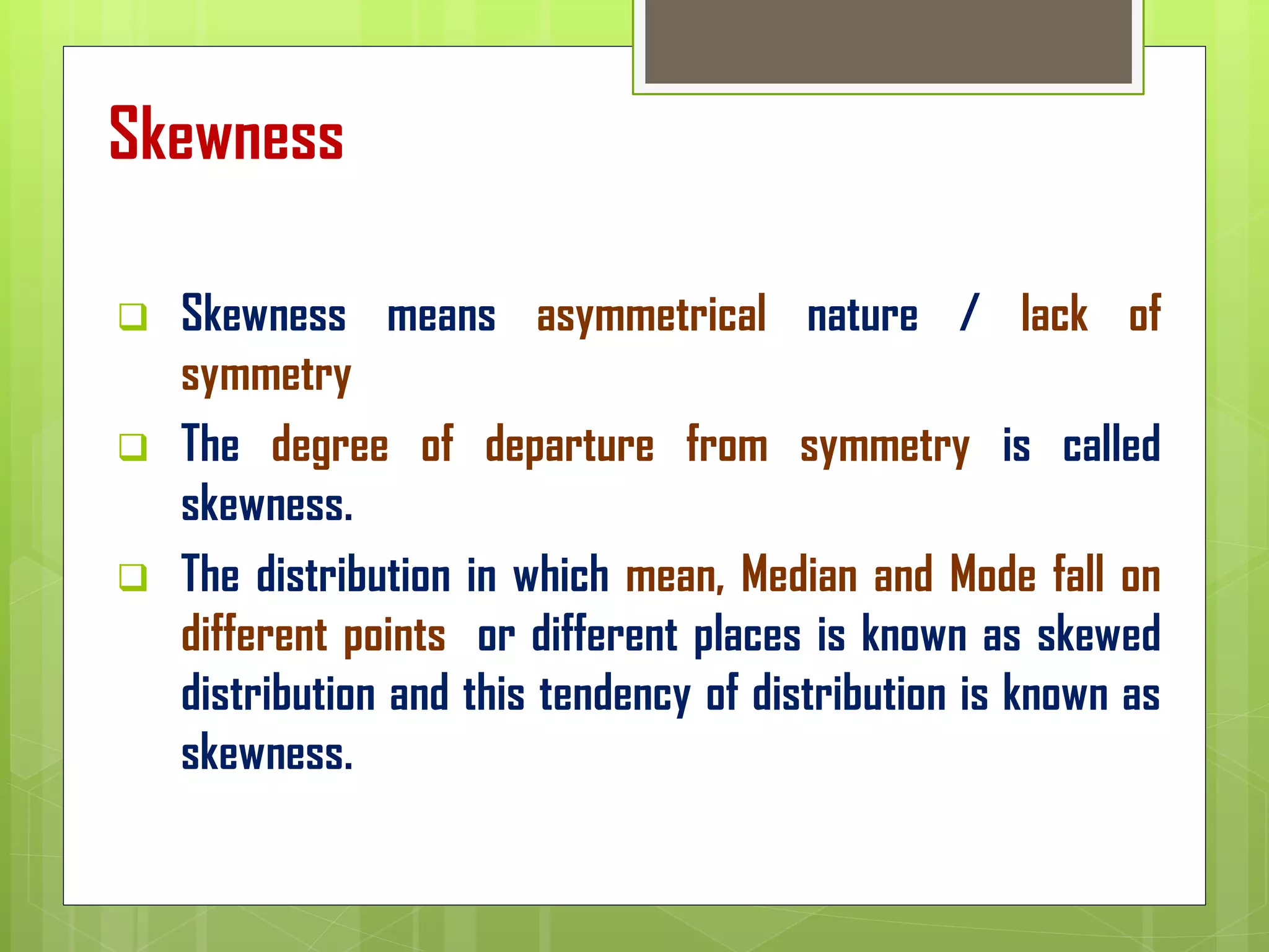
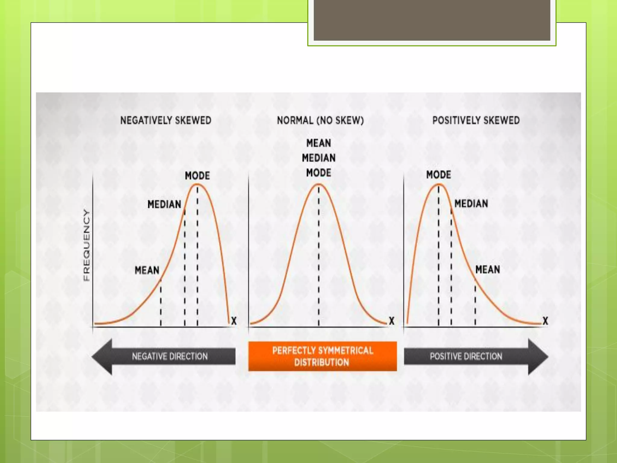
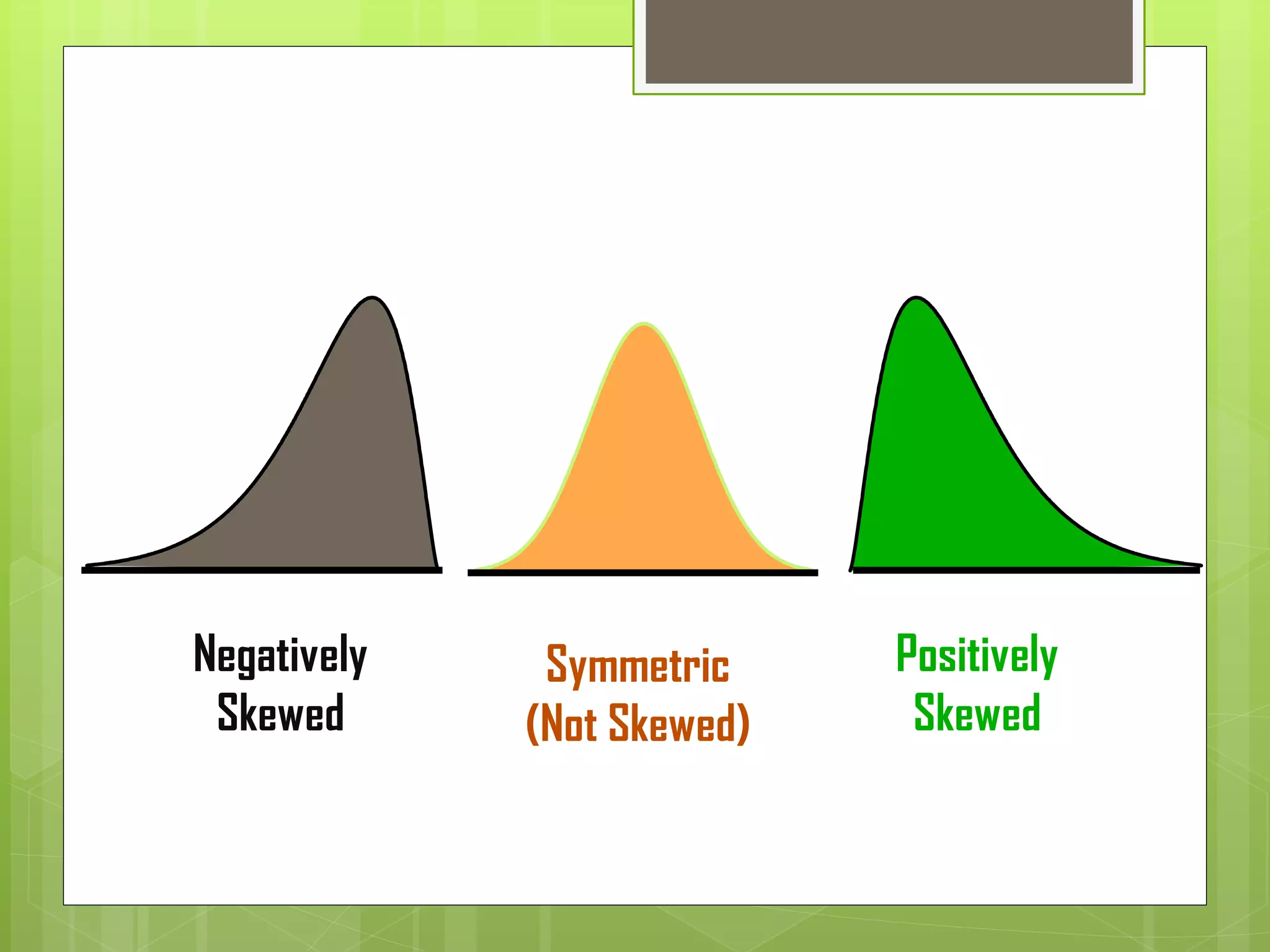
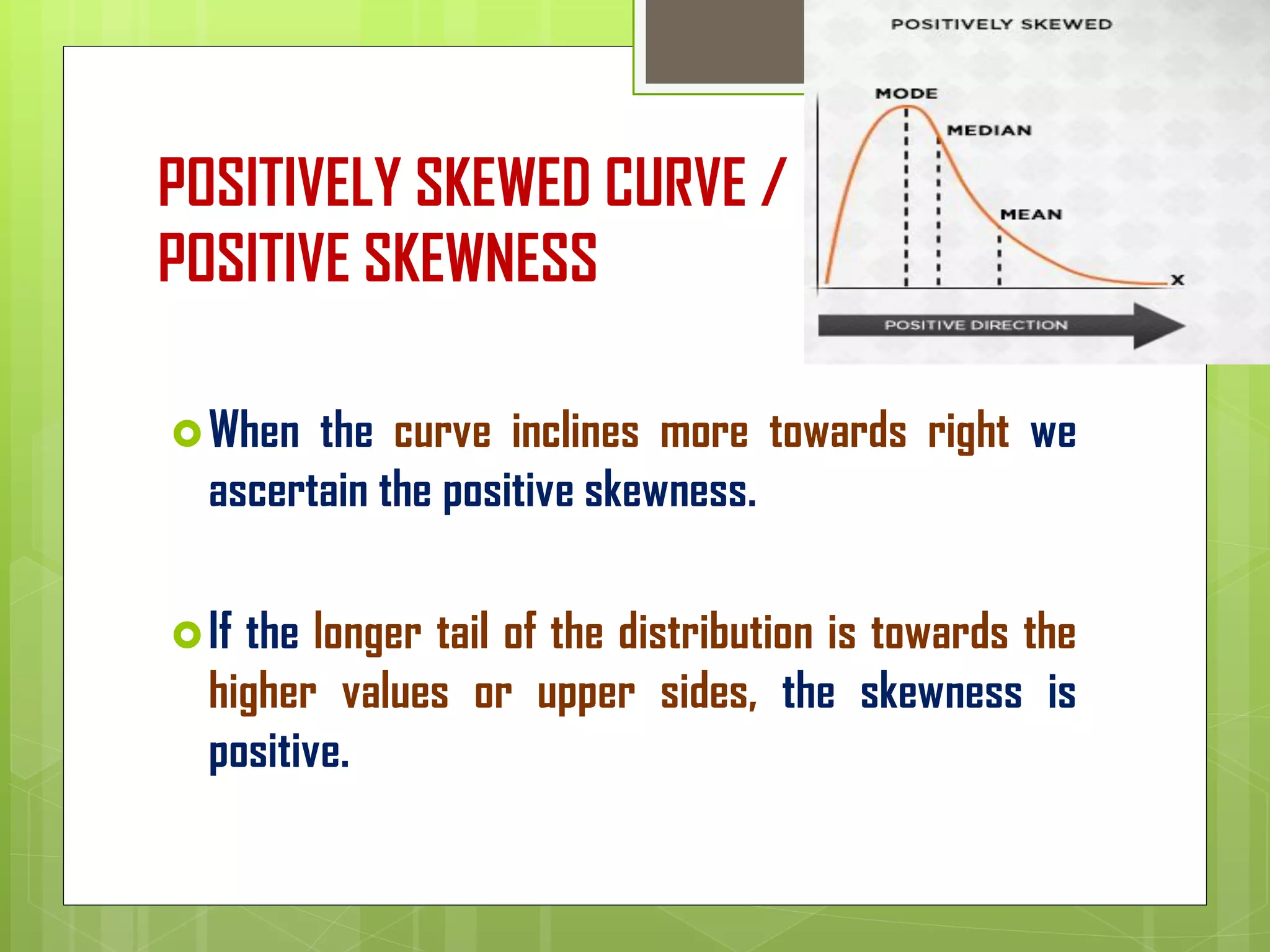
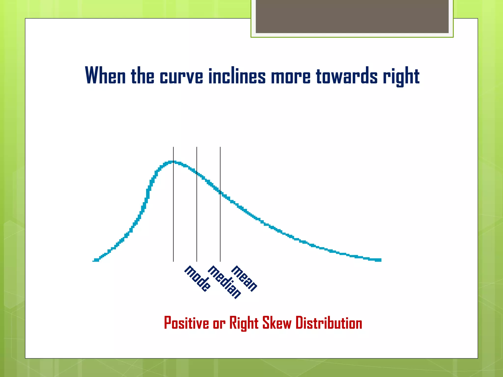
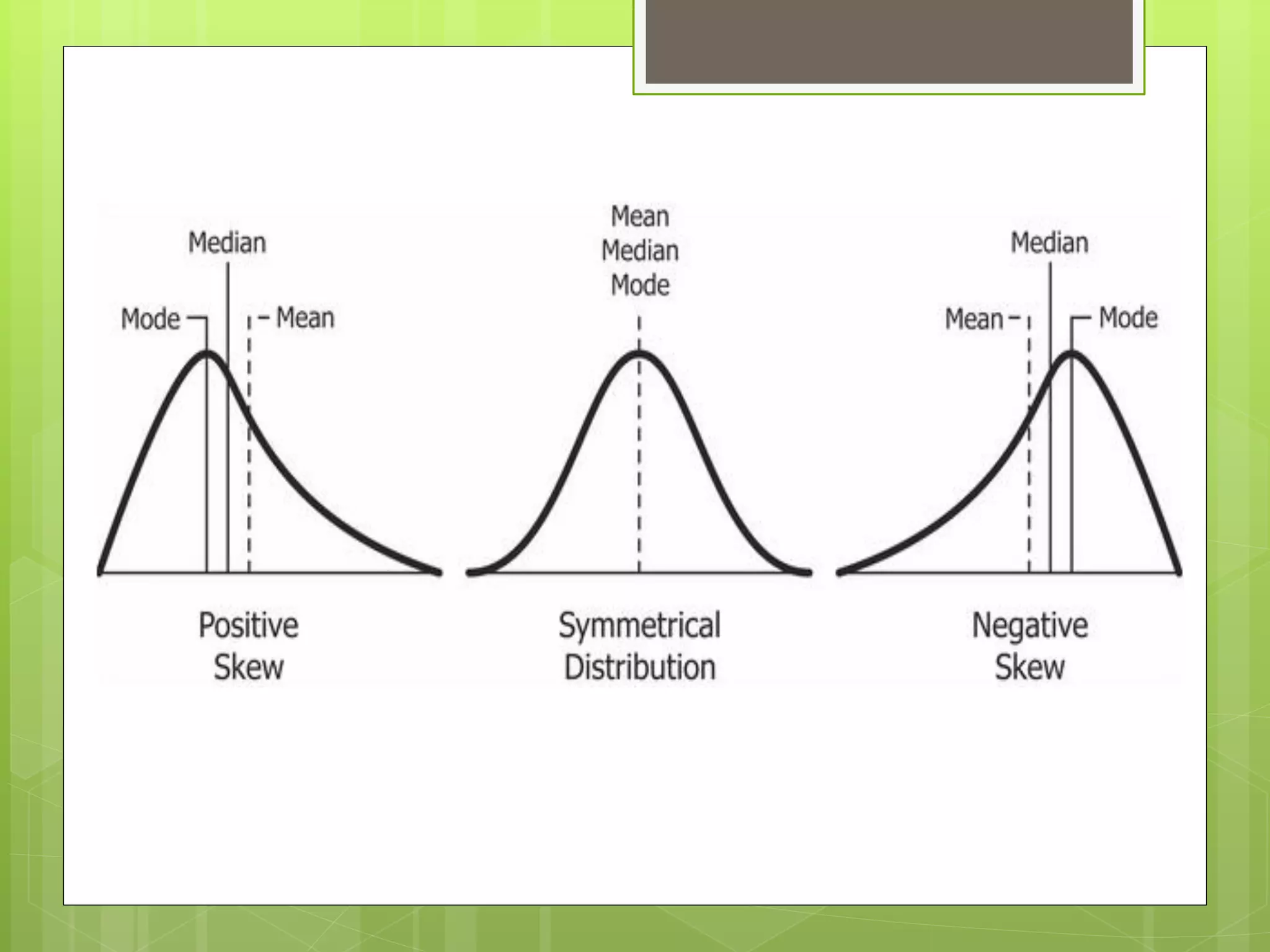

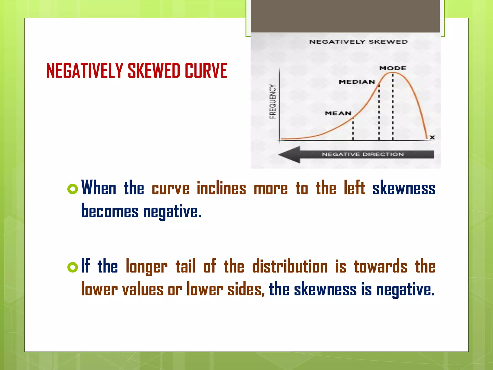
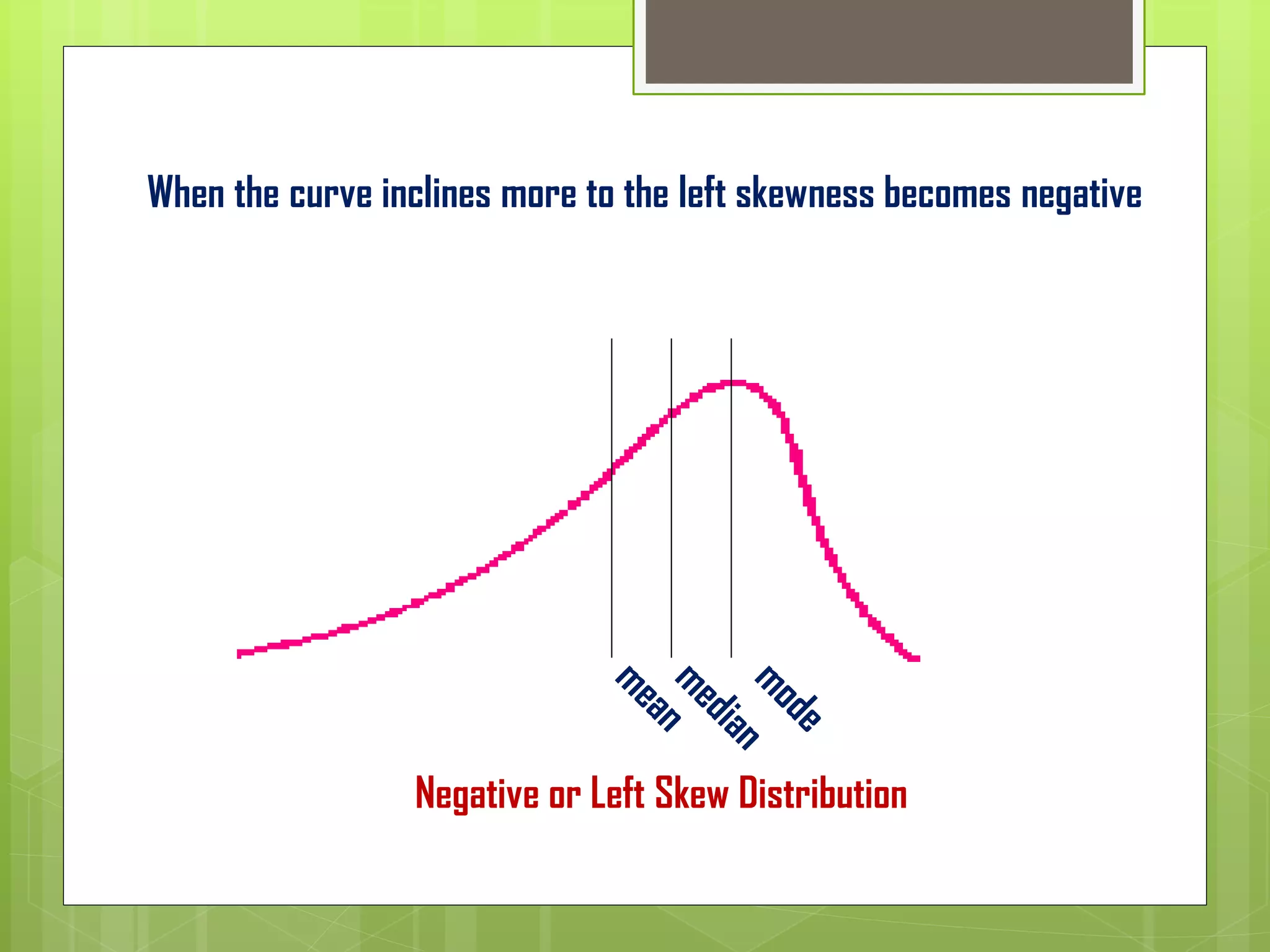

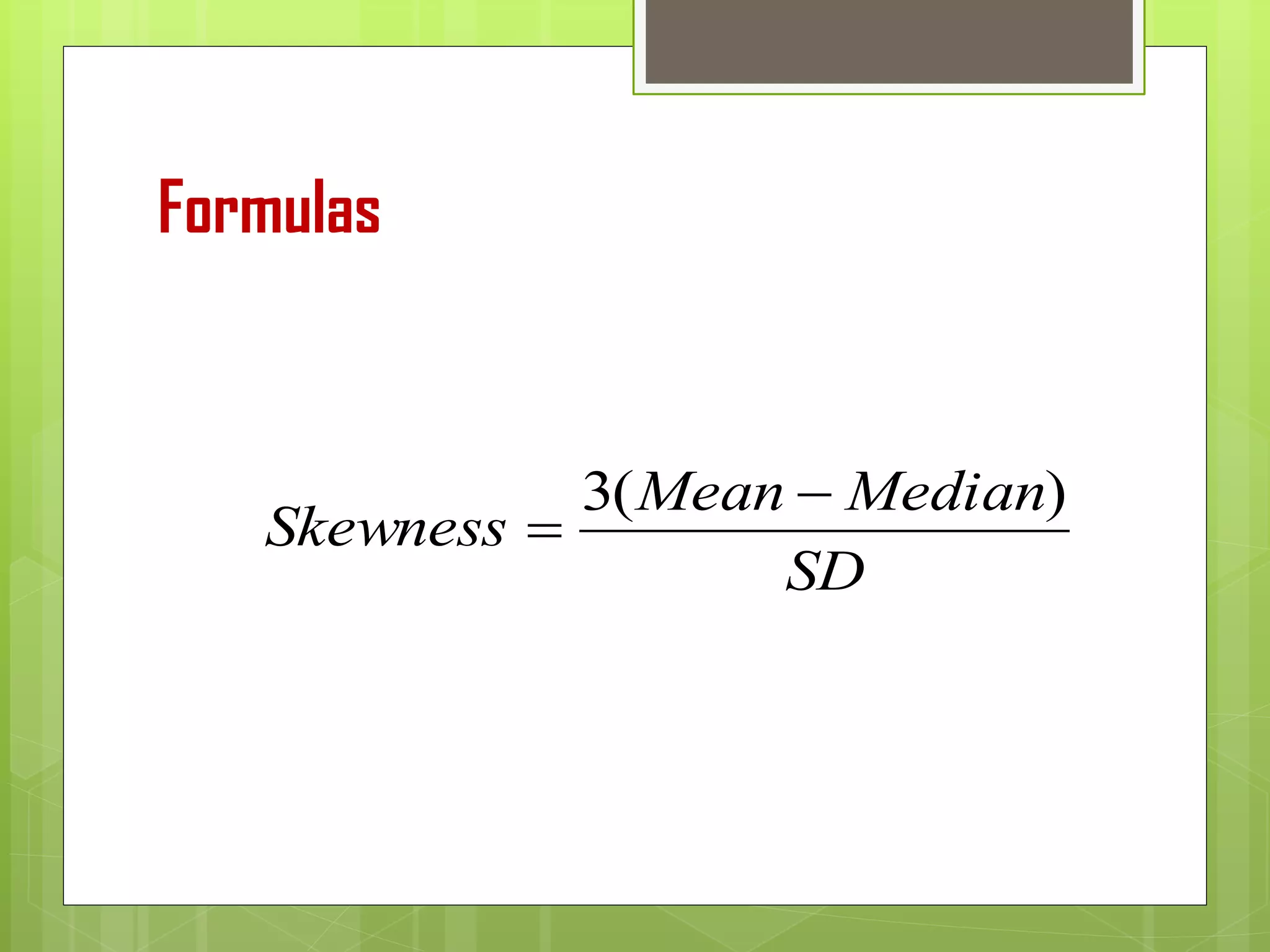
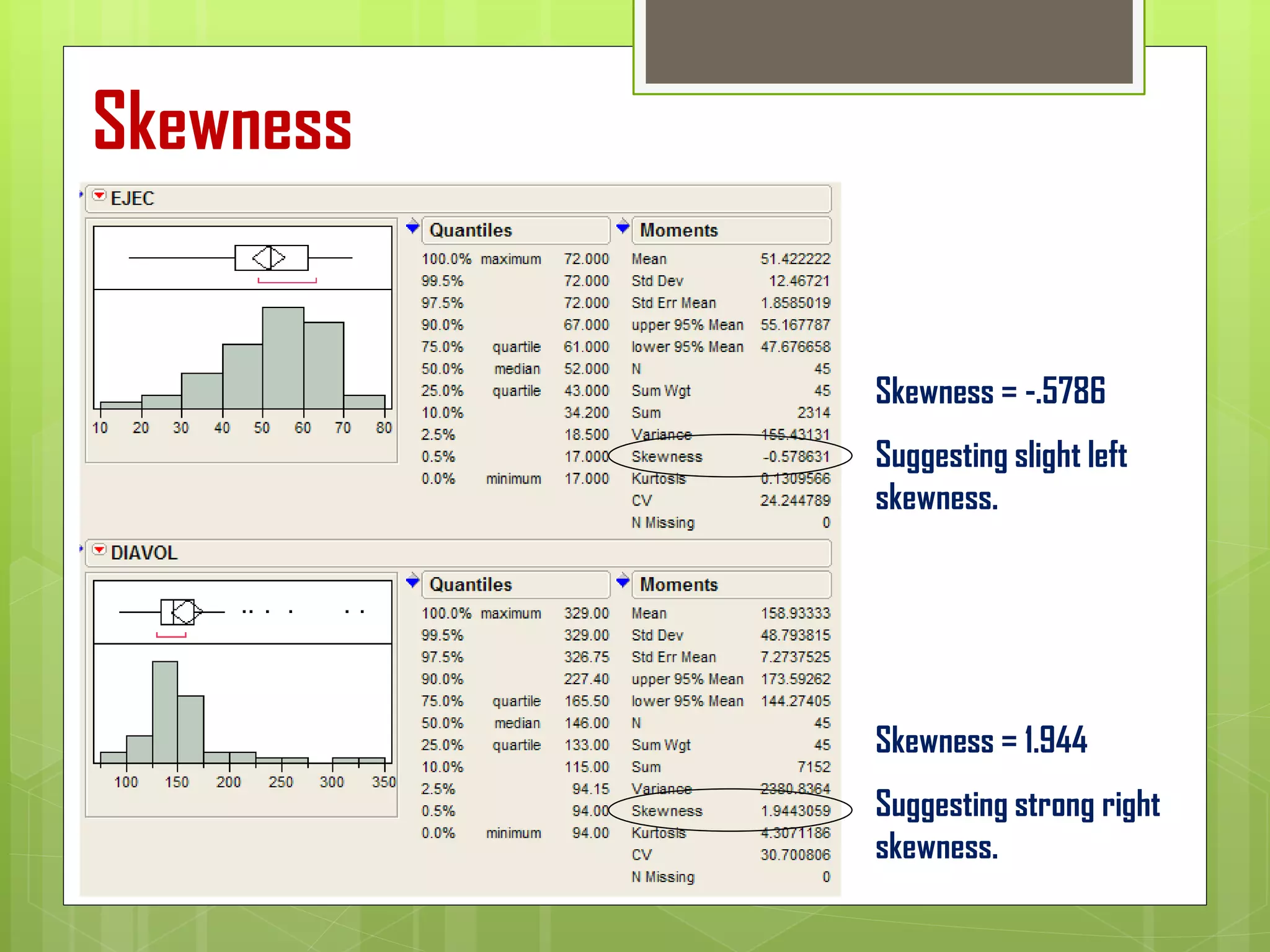
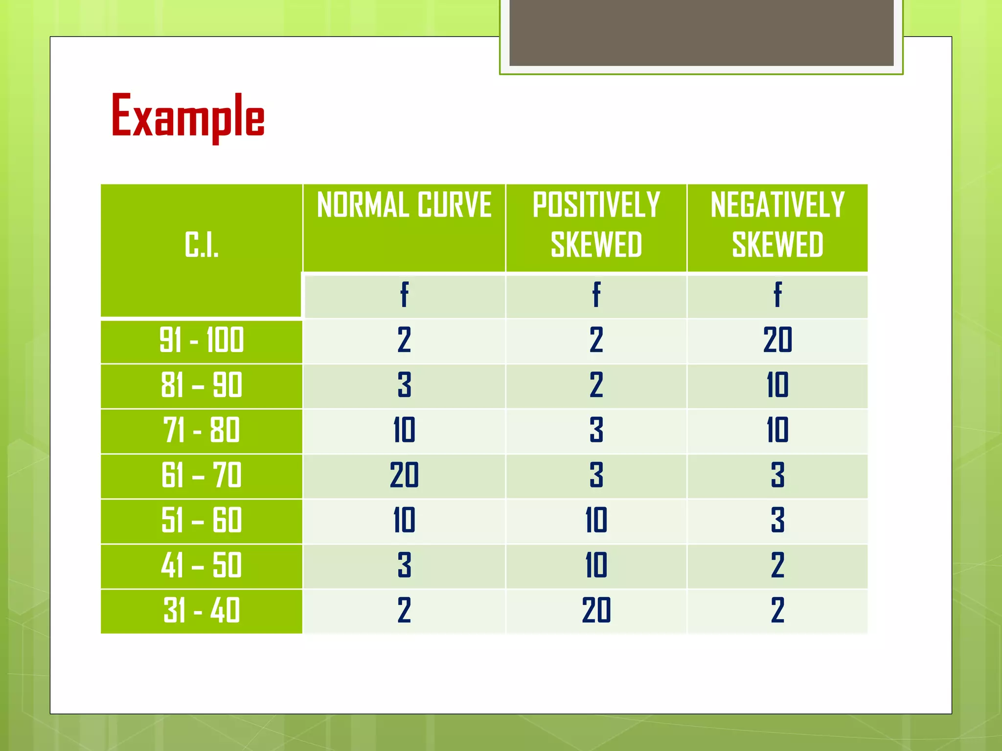
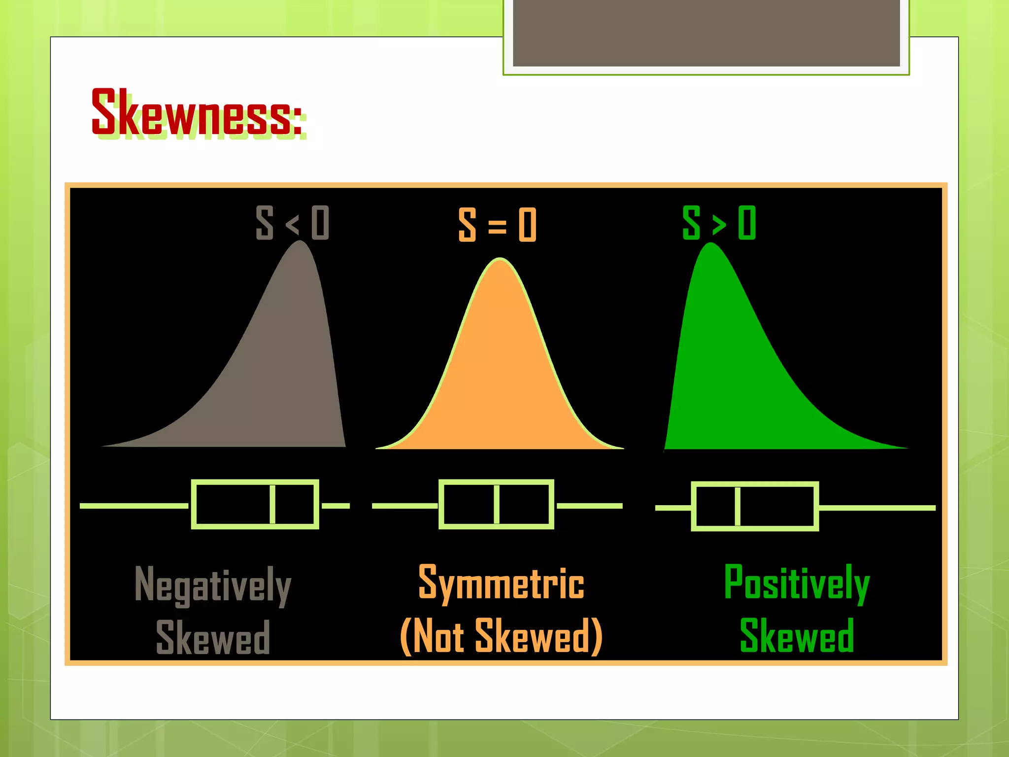

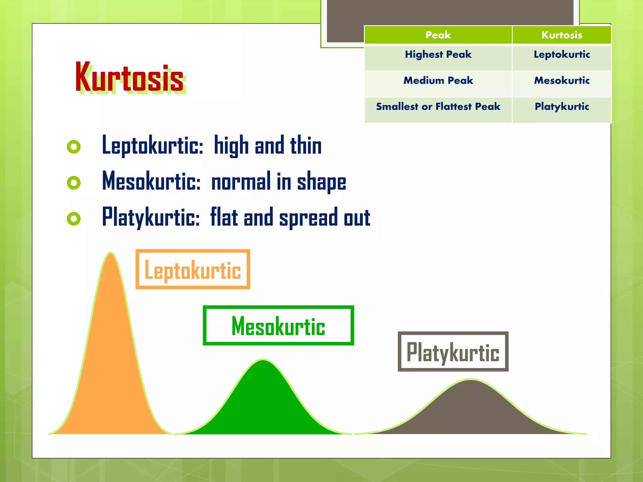
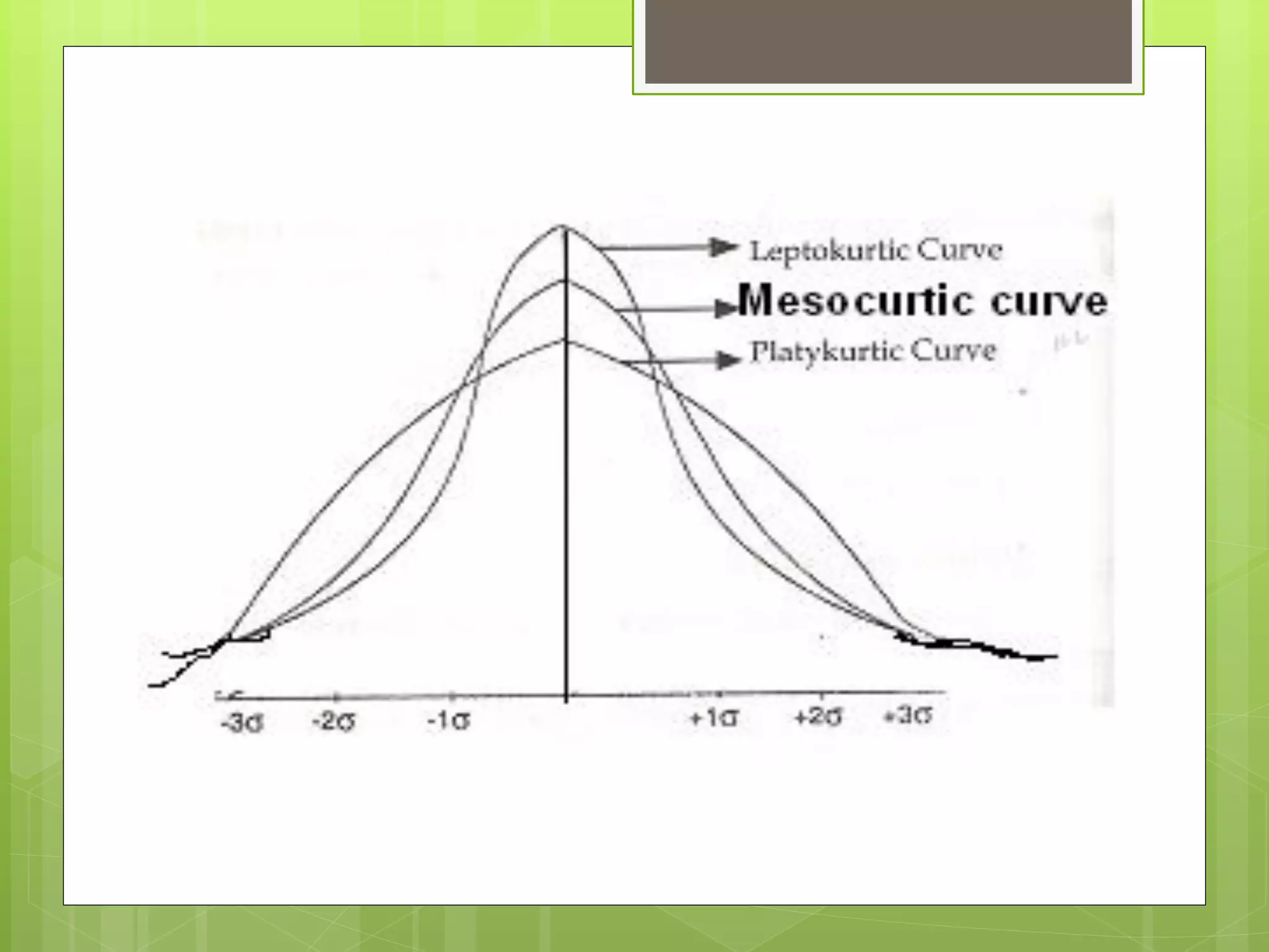
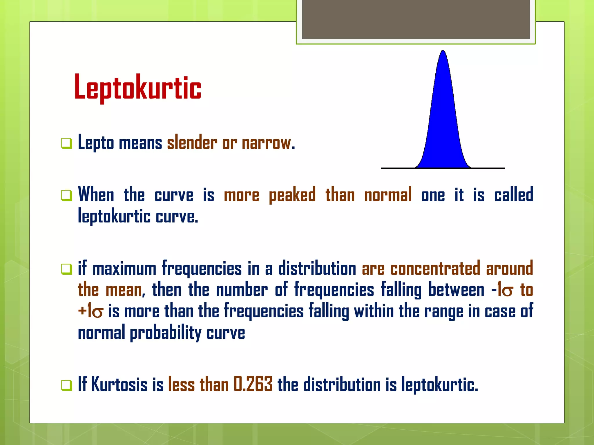

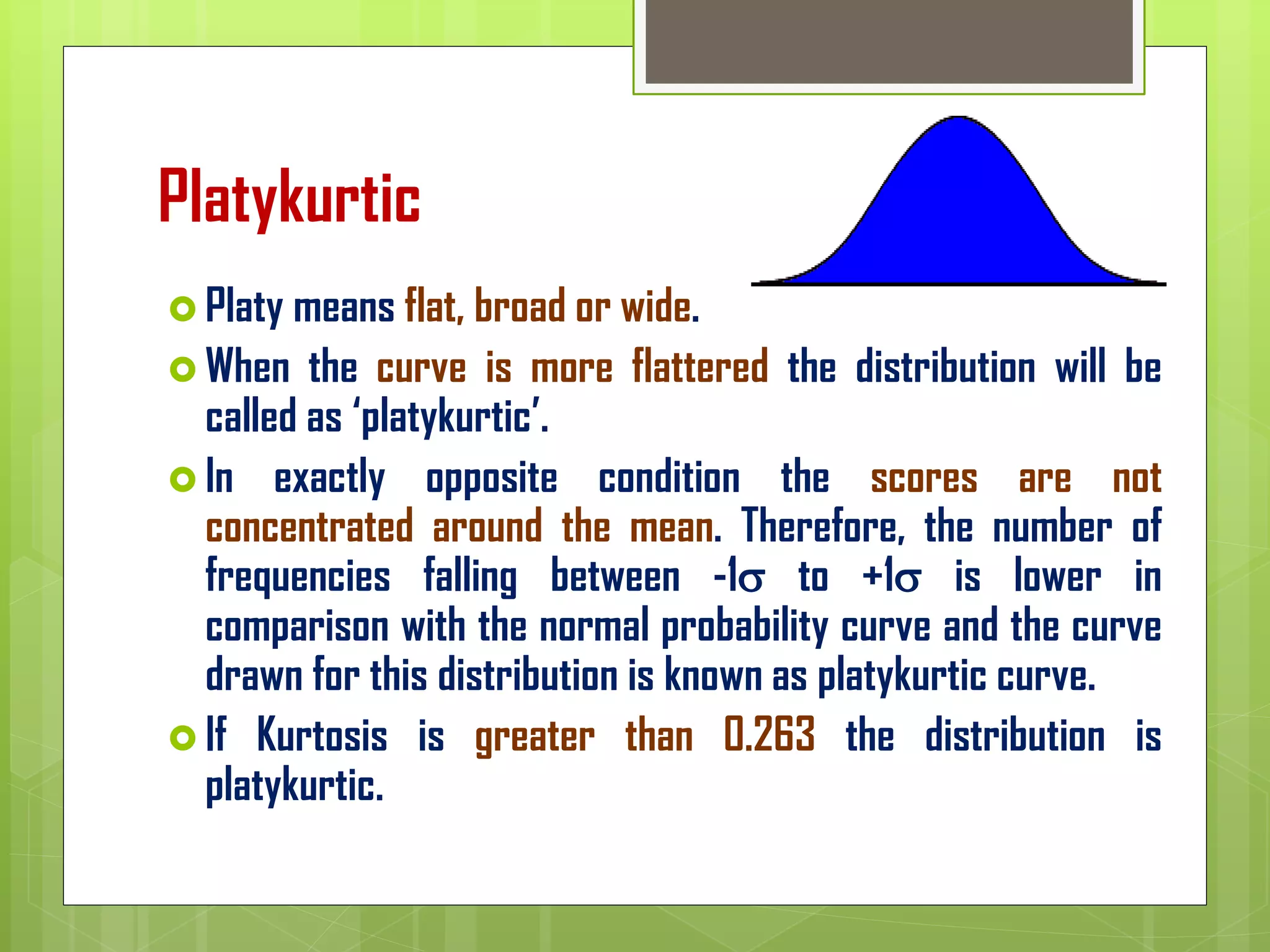


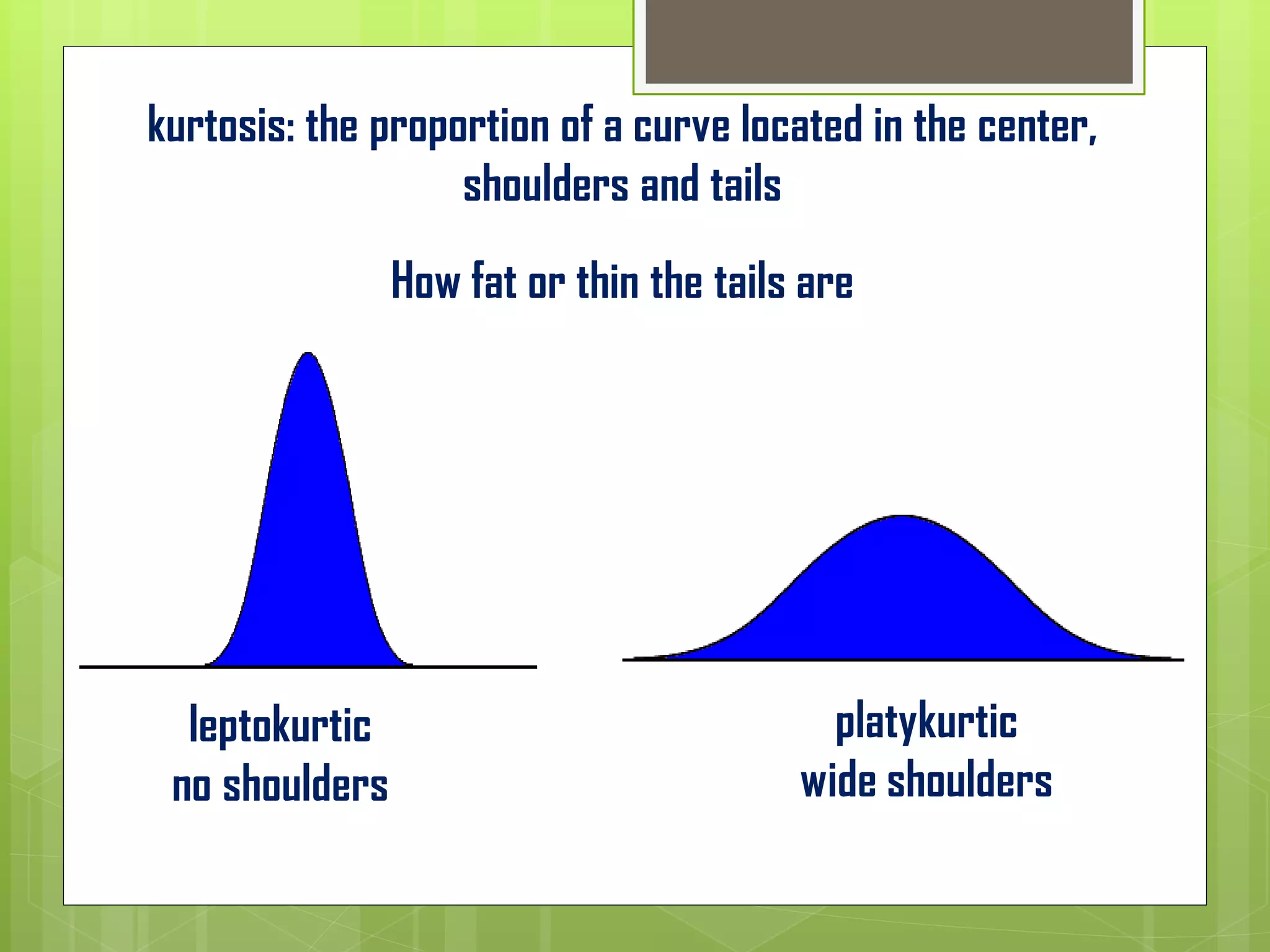


The document discusses properties of the normal probability distribution or "normal curve". It describes: 1) The normal curve is bell-shaped and symmetrical about the mean, with the mean, median and mode falling at the same point. 2) Approximately 68% of the values fall within one standard deviation of the mean, 95% within two standard deviations, and 99.7% within three standard deviations, according to the empirical rule. 3) Skewness measures asymmetry - a curve can be positively skewed if the tail extends toward higher values, negatively skewed if the tail extends toward lower values, or symmetrical. 4) Kurtosis measures peakedness - a distribution can be platykurtic