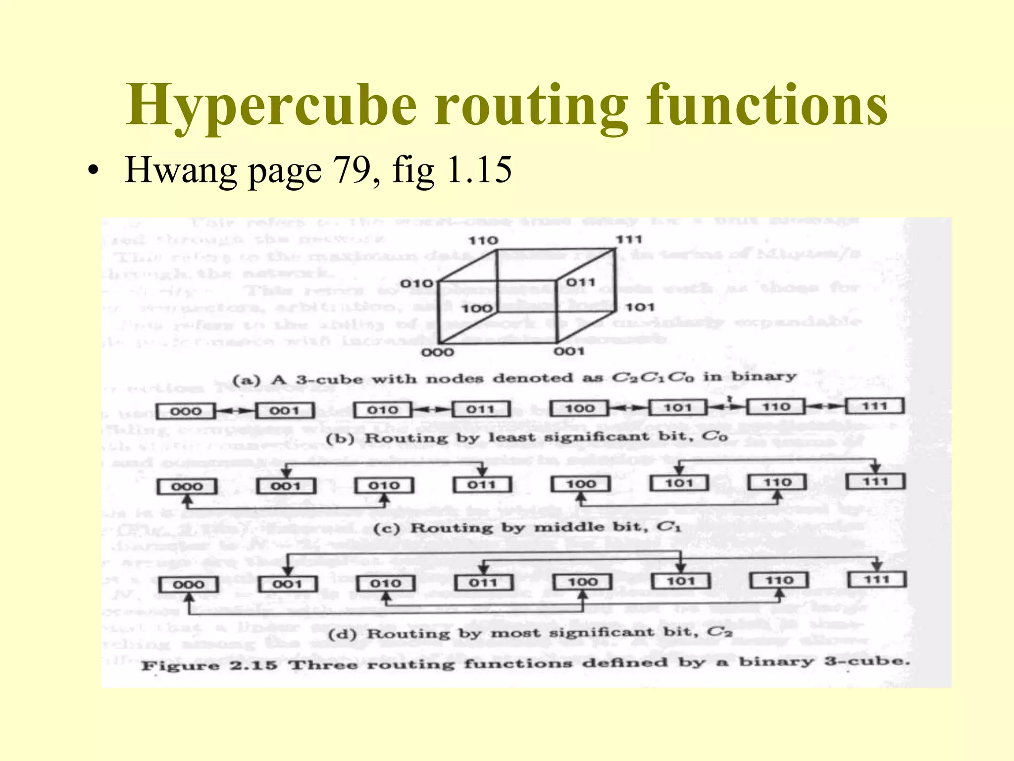
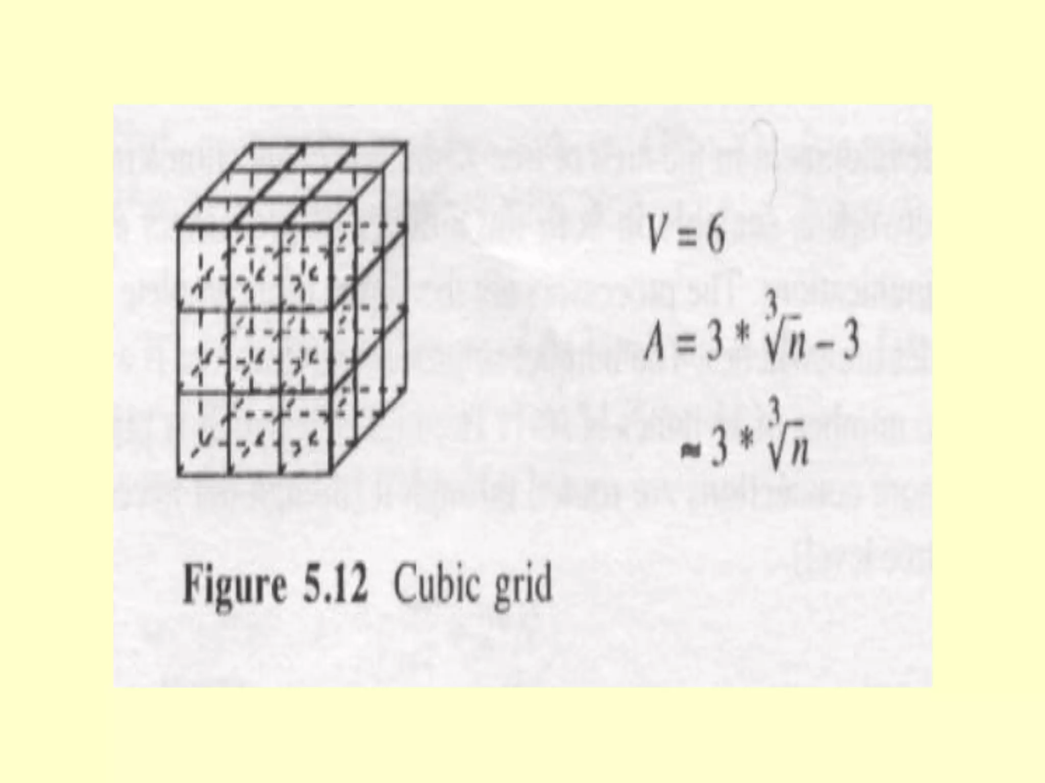
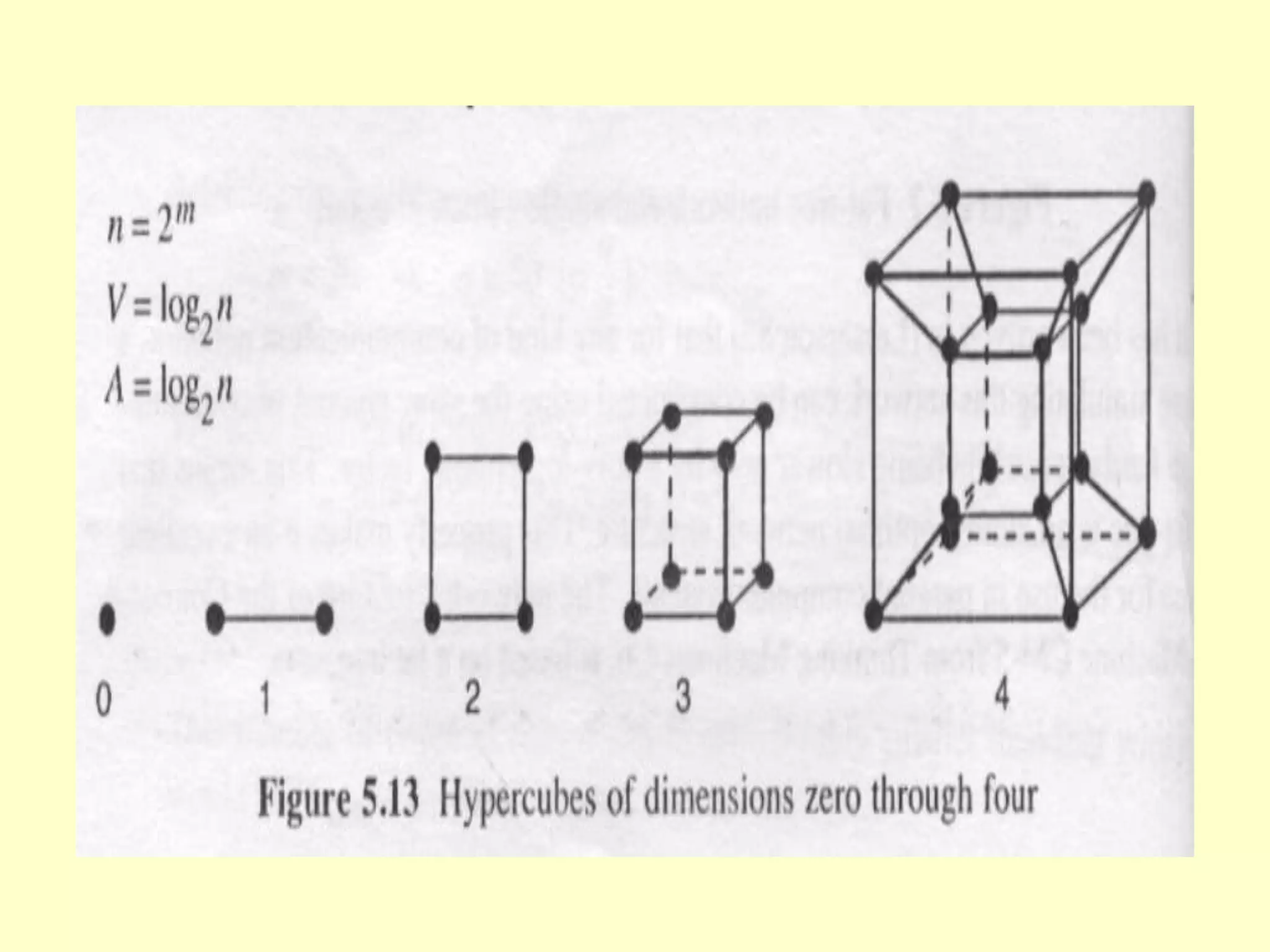
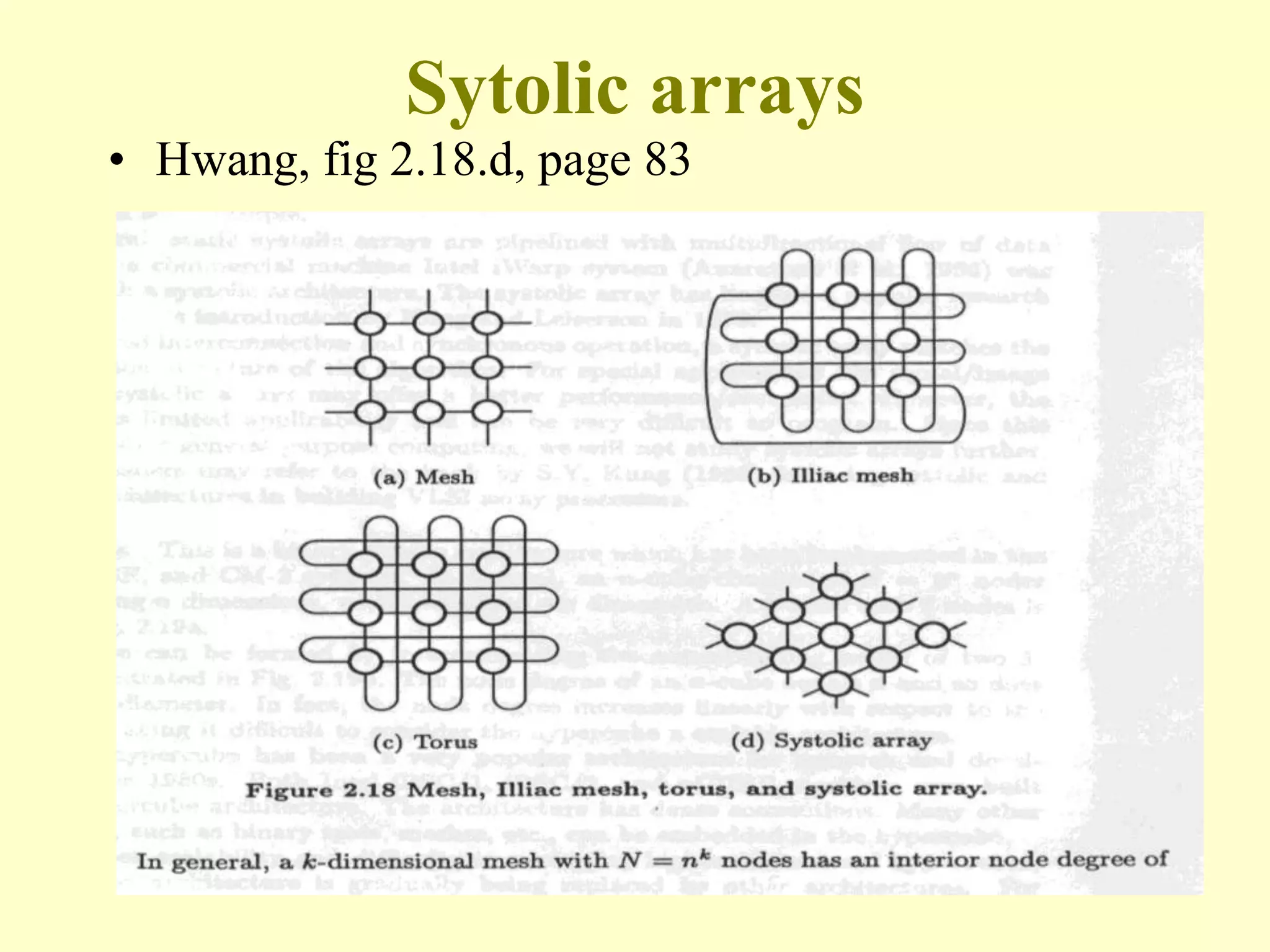
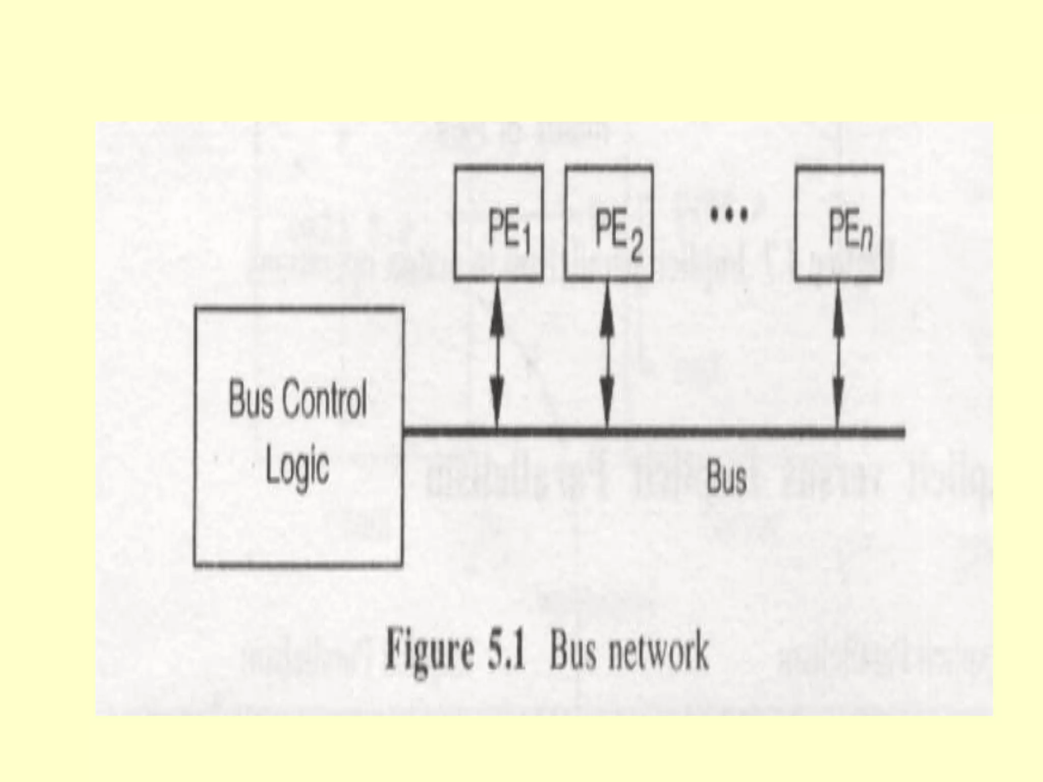
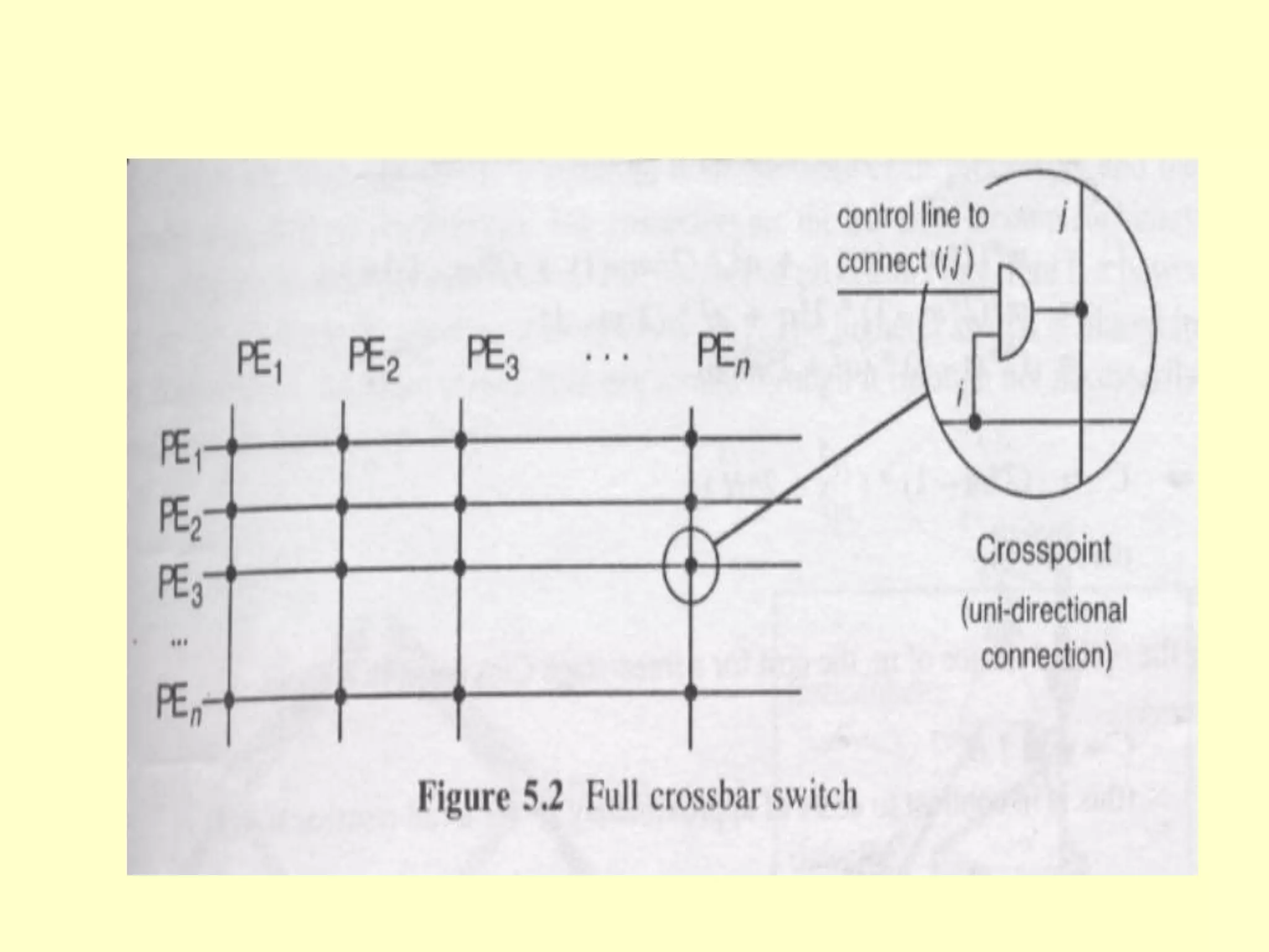
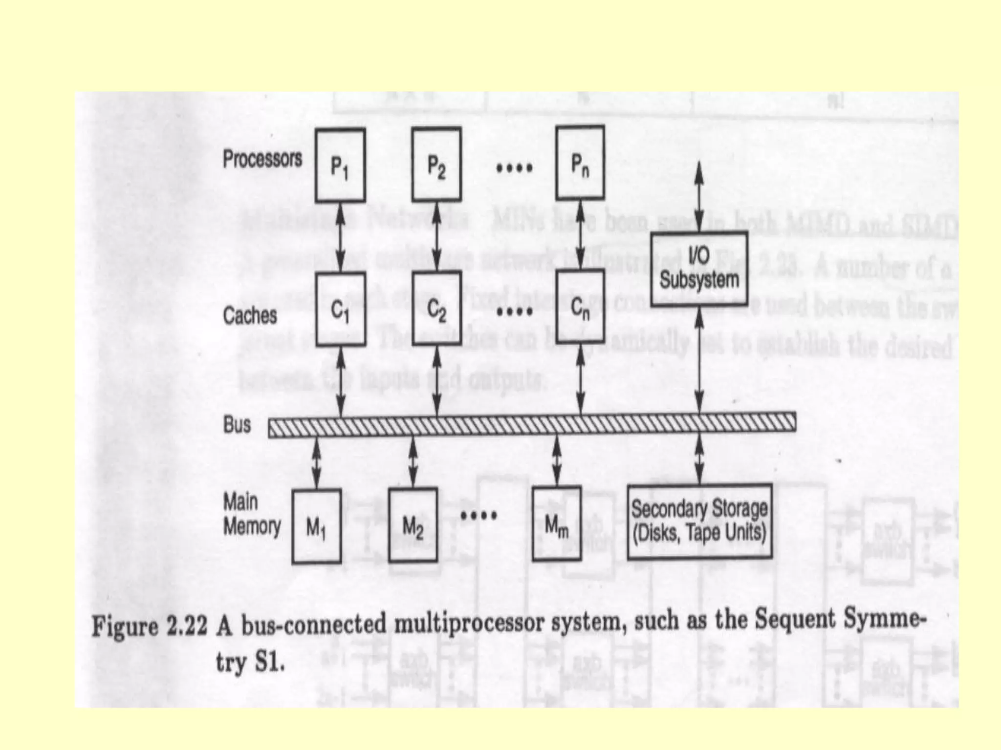
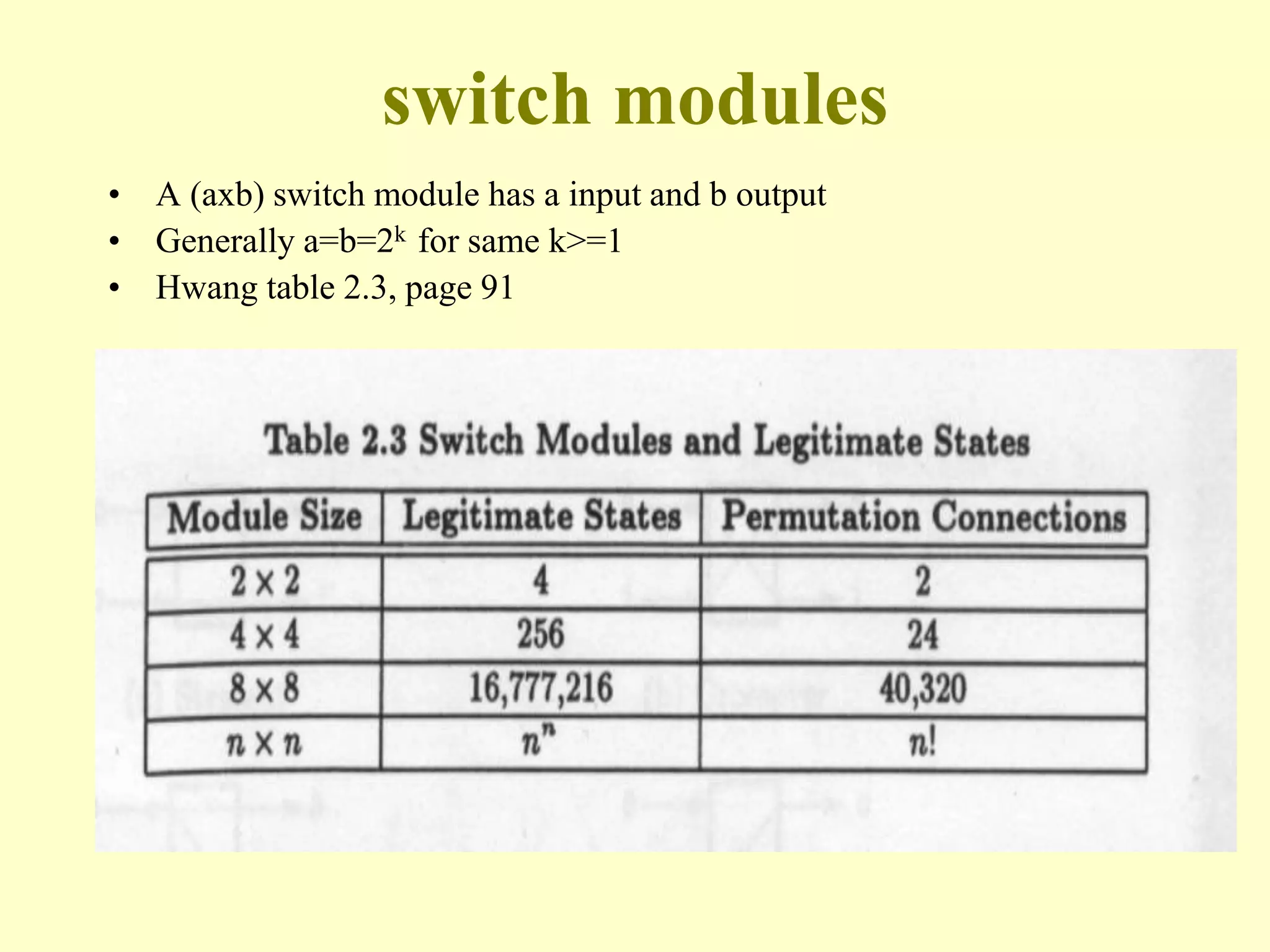
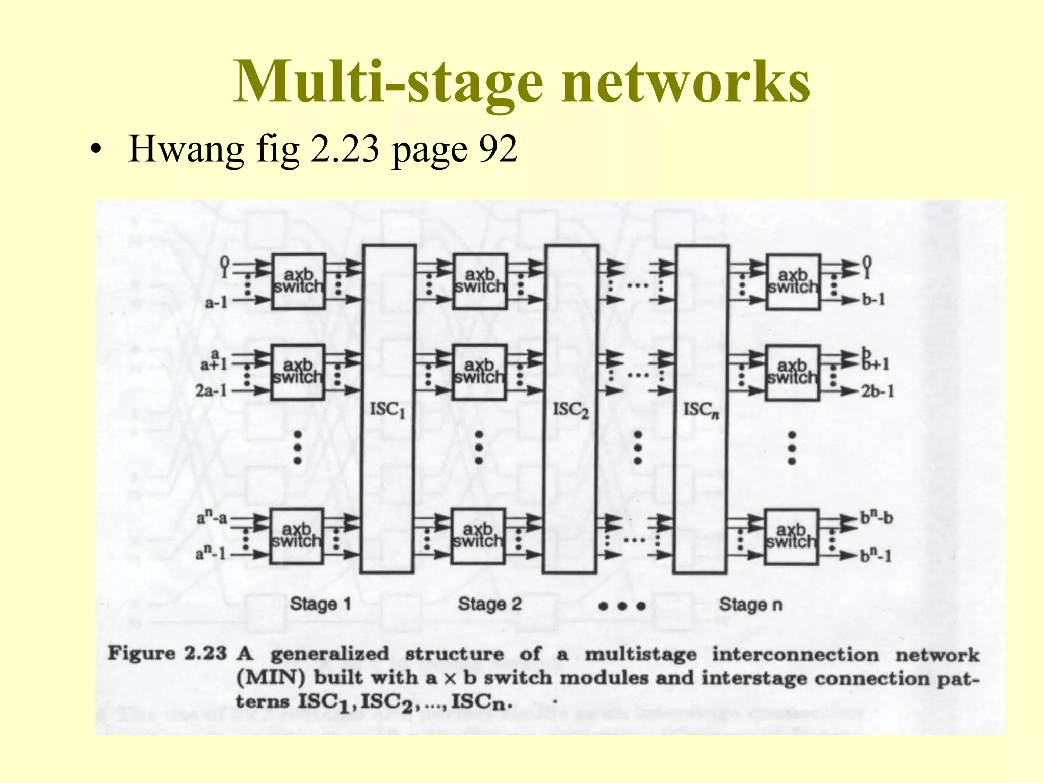
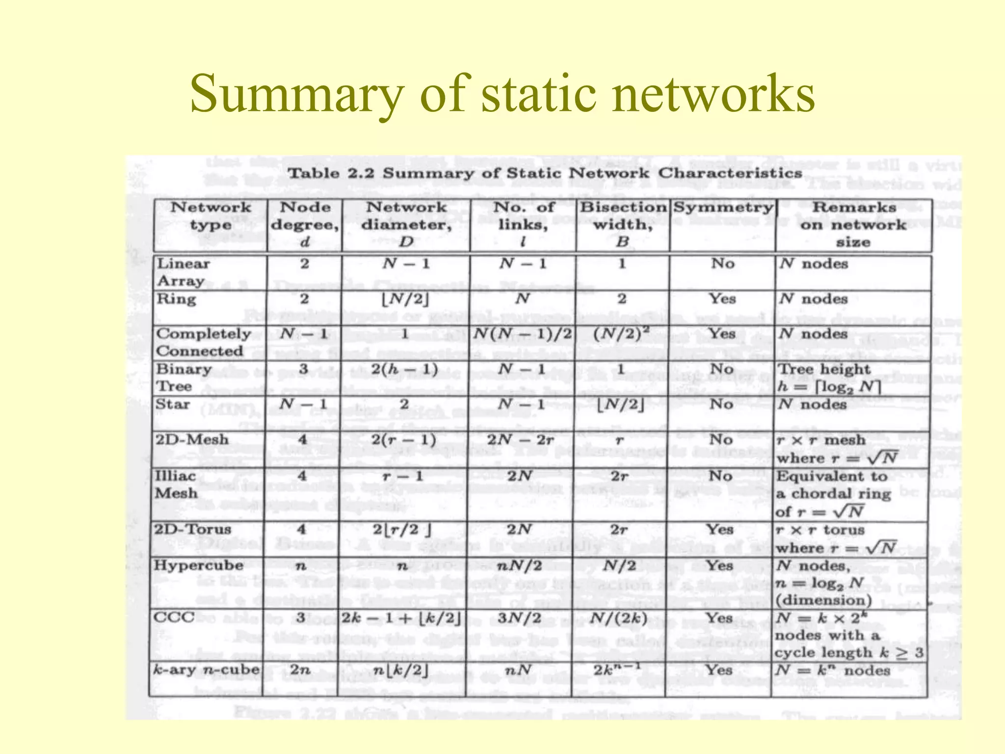
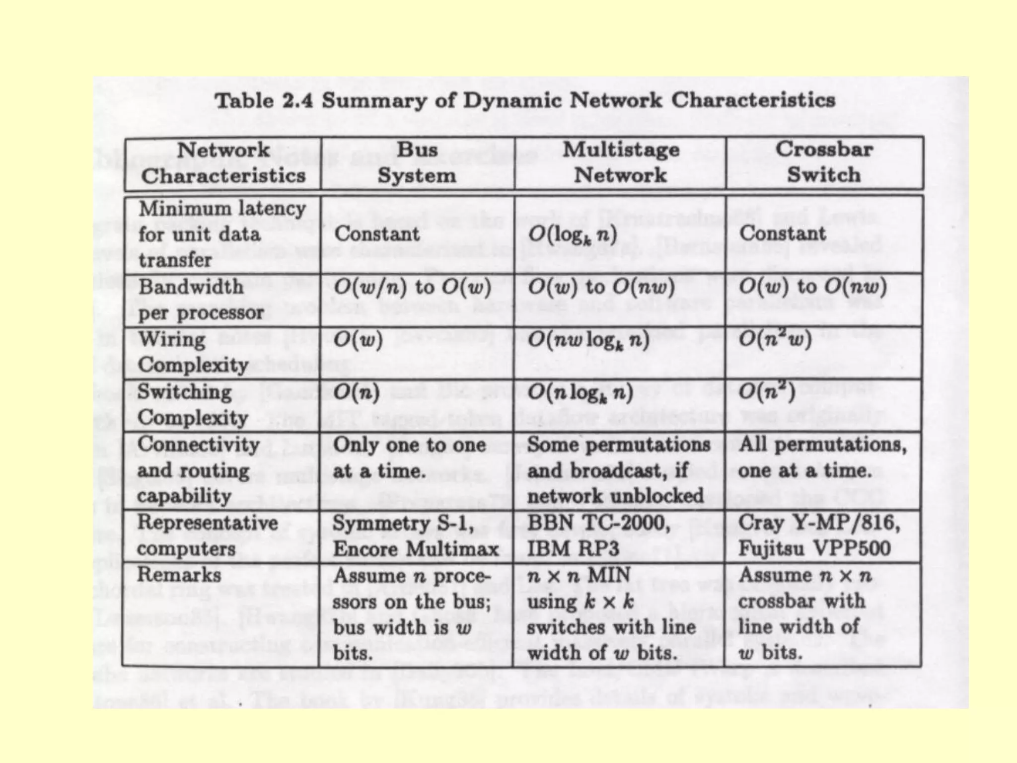
Chapter 5
Network Structures
Chapter 5
Network Structures
• 5.1 Introduction
• 5.2 System interconnection architectures
• 5.3 Network properties and routing; Node degree and
Network diameter; Node degree, Network diameter, Average
Distance and Bisection width
• 5.4 Data routing functions; Perfect shuffle and
exchange, Hypercube routing function, Broadcast and
Multicast and Network throughput
• 5.5 Network performance
• 5.6 Static networks ; Point to point Networks>
Binary Tree, ternary tree and quadtree, Fat tree,
Linear arrays, Rings, Complete graph, Grid and
Torus, AMP (A Minimum Path Systems and
Hexagonal Grid
• 5.7 Dynamic networks; Bus networks and Switch
networks> Switch modules, Multi-stage
networks, Delta networks or Omega
networks, Closs networks and Crossbar networks
• 5.8 Comparison of networks
5.1 Introduction
• Every parallel computers contains a set of processors and
one or more memory modules
• These functional units must be connected with another by
some type of network.
• High level communication; shared memory (virtual or
shared) or exchange message.
• Network structure should have sufficiently high
connectivity (without ant intermediate stations
(connections)).
• There are number of limitations constraining the physical
construction of the network.
• Number of connection lines per processors is limited.
• Cost on n Pes
– a) Number of connection per PE (production cost,
network throughput)
– b) Average Distance between the PEs (network
diameter, operating cost)
• Distance must be low at acceptable level.
• The connection structure should be scaleable (from smaller
to larger.)
• Network structures are divided into three major classes.
– 1 Bus Networks
– 2 Switching networks
– 3 Point to point networks
• Another classification is
– 1 static networks
– 2 Dynamic networks
5.2 System interconnection
architectures
• Static and dynamic networks are used to connect computer
sub system of to construct a parallel system.
•
• connect disk, memory, I/O and etc.
• Various topologies are specified
• Scalability,
• low latency, high data transfer,
• communication bandwidth.
5.2 Network properties and
routing
• Static networks are formed of point-to-point direct
connections (fixed connection)
• Dynamic networks are implemented with switched
channels (changing connection).
• Before analyze various topology, let us define several
parameters used to estimate complexity, efficiency, and
cost of network.
Node degree and Network
diameter
• Node degree
• The number of edges ( links or channels) incidents on a
node called the node degree d. (in degree, out degree)
Network diameter
• Network diameter
• The Diameter D of a network is the maximum shortest
path between any two nodes. ( The length is measured by
number of links traversed)
•
• To construct minimum path is to minimize network
diamter
• Dmax , diameter of interconnection network, to minimize
number of links a message has to travel between any
source processor and other destination within the
configuration. ( at the expense of the loss of regularity in a
system)
Average Distance
• The average inter-processor distance, davg is the number of
links on average that message to traverse between a source
and a destination processor.
• The average distance for the n processors for a
configuration of diameter dmax will be determined.
•
• p=1
n ( d=1
dmax d * Npd)/ (n-1)
• Davg = ------------------------------------
• n
•
• Npd is the number of distance d away from processor p.
Bisection width
• When a network is cut into two equal halves, the minimum
number of edged ( channels) along the cut is called channel
bisection.
•
• Wire bisection width is B = bw.
•
• Channel with w = B/w
5.4 Data routing functions
• Data routing achieved through message passing.
•
• There are same primitive routing functions on a network.
•
• These are shifting, rotation, permutation (one-to-one),
Broadcast (one to all), multicast (many to many),
personalized communication (one to many), shuffle,
exchange, etc.
Perfect shuffle and exchange
• Hwang page 78, fig 2.14
Hypercube routing functions
• Hwang page 79, fig 1.15
Broadcast and Multicast
• Broadcast and Multicast
• Can be easily achieved on SIMD computers using
broadcast bus.
• Broadcast on a message passing system requires same
other mechanism ( spanning tree, flooding)
Network throughput
• Is defined as total number of messages can be handled per
unit time.
• number of message can be in the network an once.
• a hot spot can degrade performance of the entire network
by causing congestion.
• Low dimensional networks reduce contention because
having a few high-bandwidth channels results in more
resource sharing.
5.5 Network performance
• Network performance effected by some factors that summarized
below;
– 1 Functionality; How network supports data routing,
interrupt handling, synchronization, request
message/combing, and coherence.
– 2 Network latency; This refer worse case time delay for
a unit message to be transferred through network.
– 3 Bandwidth; This refers to the maximum data transfer
rate in terms of Mbytes/s transmitted through network.
– 4 Hardware complexity; This refers to implementation
cost such those for wires, switches, connectors,
arbitration, and interface logic.
– 5 Scalability; This refers to the ability of network to be
modularly expandable with a scalable performance with increasing
machine resource.
5.6 Static networks
• Static networks use direct links which are fixed once built.
• This type of network is suitable where communication
pattern are predictable or implementable with static
connection.
Point to point Networks
• All connections bi-drectional, (if not stated otherwise)
• There is a fixed connection between nodes.
•
• n : Number of PEs in the network
• V : connection for each PE
• A or D : Maximum distance between PEs.
Binary Tree, ternary tree and
quadtree
• Brunnel, Figure 5.14 and 5.15, page 48.
Fat tree
• Brunnel, fig 5.7, page 44.
Linear arrays
• Hwang fig 2.16.a, page 81
Rings
• Brunnel, Figure 5.8, page 45.
Complete graph
• Brunnel, Figure 5.9, page 45.
Grid and Torus
• Brunnel, Figure 5.10, page 46.
AMP (A Minimum Path Systems)
• Alan, page 30, fig 21
Hexagonal Grid
• Brunnel, Figure 5.11, page 46.
• Cube and hypercube
• Brunnel, Figure 5.12 and 5.13, page 47.
Sytolic arrays
• Hwang, fig 2.18.d, page 83
5.7 Dynamic networks
• For multipurpose and general purpose.
• Communication pattern based on program demands.
• Bus systems, multi stage inter connections, crossbar switch
networks,
• Cost depends on wiring,
• Performance depend on network bandwith, data transfer
rate, network latency and communication pattern
supported.
Bus networks
• cheap
• simple
• optimal (??)
• common (networks, LANs)
• Bandwidth remains fixed and divided by users.
• One transaction at a time.
– 1 Contention and,
– 2 Time sharing bus.
• Von Neumann model connects all processor and memory
modules and other modules.
• Brunnel , (fig 5.2, page 39)
• Hwang, ( fig 2.22, page 90)
• Parallel reading possible same location but writing is not.
• Parallel reading and writing to different memory locations
are not possible.
• Bust controller must control the access of the bus
– 1 centralized and
– 2 decentralized.
Switch networks
• Dynamic connections achieved with active elements.
• Varying connection patterns can be engaged during run
time of a program.
• Crossbar switches, delta networks.
switch modules
• A (axb) switch module has a input and b output
• Generally a=b=2k for same k>=1
• Hwang table 2.3, page 91
Multi-stage networks
• Hwang fig 2.23 page 92
Delta networks or Omega
networks
• Cost reduced from n2 (switch networkte ) to k??*n
• Brunnel fig 5.4 and fig 5.5 page 41
• Hwang page 92, fig 2.224
Closs networks
• Brunnel (fig 5.6, page 42,)
Crossbar networks
• Each PE has n cross points.
• total network with n PEs has n2 cross point.
• any connection permutation can be specified
• collision free.
• Fully parallel information exchange can be performed.
• Highest bandwidth and interconnection capability are
provided by crossbar networks
• Same module (memory) multiple request at the same time
one request satisfied.
• Brunnel, Fig 5.2 page 40.
• Hwang figure 2.26, page 94.
5.8 Comparison of networks
• Summary of static networks
• Symmetry affect scalability and routing efficiency.It s fair
to say that the total network cost increases with d (degree)
and l (links).
• Hwang, table 2.2, page 88
• The best solution for a particular system is a function of the
system’s intended application, size, speed requirements,
cost requirements, etc.
• global communication are generally interested rather than
local.
Summary of static networks
Summary of dynamic networks
• A summary comparison of dynamic networks is given
figure below
• (Hwang table, 2.4 page 95)
BIL406-Chapter-5-Network Structures.ppt

BIL406-Chapter-5-Network Structures.ppt

  • 1.
  • 2.
    Chapter 5 Network Structures •5.1 Introduction • 5.2 System interconnection architectures • 5.3 Network properties and routing; Node degree and Network diameter; Node degree, Network diameter, Average Distance and Bisection width • 5.4 Data routing functions; Perfect shuffle and exchange, Hypercube routing function, Broadcast and Multicast and Network throughput
  • 3.
    • 5.5 Networkperformance • 5.6 Static networks ; Point to point Networks> Binary Tree, ternary tree and quadtree, Fat tree, Linear arrays, Rings, Complete graph, Grid and Torus, AMP (A Minimum Path Systems and Hexagonal Grid • 5.7 Dynamic networks; Bus networks and Switch networks> Switch modules, Multi-stage networks, Delta networks or Omega networks, Closs networks and Crossbar networks • 5.8 Comparison of networks
  • 4.
    5.1 Introduction • Everyparallel computers contains a set of processors and one or more memory modules • These functional units must be connected with another by some type of network. • High level communication; shared memory (virtual or shared) or exchange message. • Network structure should have sufficiently high connectivity (without ant intermediate stations (connections)). • There are number of limitations constraining the physical construction of the network. • Number of connection lines per processors is limited.
  • 5.
    • Cost onn Pes – a) Number of connection per PE (production cost, network throughput) – b) Average Distance between the PEs (network diameter, operating cost) • Distance must be low at acceptable level. • The connection structure should be scaleable (from smaller to larger.) • Network structures are divided into three major classes. – 1 Bus Networks – 2 Switching networks – 3 Point to point networks • Another classification is – 1 static networks – 2 Dynamic networks
  • 6.
    5.2 System interconnection architectures •Static and dynamic networks are used to connect computer sub system of to construct a parallel system. • • connect disk, memory, I/O and etc. • Various topologies are specified • Scalability, • low latency, high data transfer, • communication bandwidth.
  • 7.
    5.2 Network propertiesand routing • Static networks are formed of point-to-point direct connections (fixed connection) • Dynamic networks are implemented with switched channels (changing connection). • Before analyze various topology, let us define several parameters used to estimate complexity, efficiency, and cost of network.
  • 8.
    Node degree andNetwork diameter • Node degree • The number of edges ( links or channels) incidents on a node called the node degree d. (in degree, out degree)
  • 9.
    Network diameter • Networkdiameter • The Diameter D of a network is the maximum shortest path between any two nodes. ( The length is measured by number of links traversed) • • To construct minimum path is to minimize network diamter • Dmax , diameter of interconnection network, to minimize number of links a message has to travel between any source processor and other destination within the configuration. ( at the expense of the loss of regularity in a system)
  • 10.
    Average Distance • Theaverage inter-processor distance, davg is the number of links on average that message to traverse between a source and a destination processor. • The average distance for the n processors for a configuration of diameter dmax will be determined. • • p=1 n ( d=1 dmax d * Npd)/ (n-1) • Davg = ------------------------------------ • n • • Npd is the number of distance d away from processor p.
  • 11.
    Bisection width • Whena network is cut into two equal halves, the minimum number of edged ( channels) along the cut is called channel bisection. • • Wire bisection width is B = bw. • • Channel with w = B/w
  • 12.
    5.4 Data routingfunctions • Data routing achieved through message passing. • • There are same primitive routing functions on a network. • • These are shifting, rotation, permutation (one-to-one), Broadcast (one to all), multicast (many to many), personalized communication (one to many), shuffle, exchange, etc.
  • 13.
    Perfect shuffle andexchange • Hwang page 78, fig 2.14
  • 14.
    Hypercube routing functions •Hwang page 79, fig 1.15
  • 15.
    Broadcast and Multicast •Broadcast and Multicast • Can be easily achieved on SIMD computers using broadcast bus. • Broadcast on a message passing system requires same other mechanism ( spanning tree, flooding)
  • 16.
    Network throughput • Isdefined as total number of messages can be handled per unit time. • number of message can be in the network an once. • a hot spot can degrade performance of the entire network by causing congestion. • Low dimensional networks reduce contention because having a few high-bandwidth channels results in more resource sharing.
  • 17.
    5.5 Network performance •Network performance effected by some factors that summarized below; – 1 Functionality; How network supports data routing, interrupt handling, synchronization, request message/combing, and coherence. – 2 Network latency; This refer worse case time delay for a unit message to be transferred through network. – 3 Bandwidth; This refers to the maximum data transfer rate in terms of Mbytes/s transmitted through network. – 4 Hardware complexity; This refers to implementation cost such those for wires, switches, connectors, arbitration, and interface logic. – 5 Scalability; This refers to the ability of network to be modularly expandable with a scalable performance with increasing machine resource.
  • 18.
    5.6 Static networks •Static networks use direct links which are fixed once built. • This type of network is suitable where communication pattern are predictable or implementable with static connection.
  • 19.
    Point to pointNetworks • All connections bi-drectional, (if not stated otherwise) • There is a fixed connection between nodes. • • n : Number of PEs in the network • V : connection for each PE • A or D : Maximum distance between PEs.
  • 20.
    Binary Tree, ternarytree and quadtree • Brunnel, Figure 5.14 and 5.15, page 48.
  • 23.
    Fat tree • Brunnel,fig 5.7, page 44.
  • 24.
    Linear arrays • Hwangfig 2.16.a, page 81
  • 25.
  • 26.
    Complete graph • Brunnel,Figure 5.9, page 45.
  • 27.
    Grid and Torus •Brunnel, Figure 5.10, page 46.
  • 28.
    AMP (A MinimumPath Systems) • Alan, page 30, fig 21
  • 29.
    Hexagonal Grid • Brunnel,Figure 5.11, page 46. • Cube and hypercube • Brunnel, Figure 5.12 and 5.13, page 47.
  • 32.
    Sytolic arrays • Hwang,fig 2.18.d, page 83
  • 33.
    5.7 Dynamic networks •For multipurpose and general purpose. • Communication pattern based on program demands. • Bus systems, multi stage inter connections, crossbar switch networks, • Cost depends on wiring, • Performance depend on network bandwith, data transfer rate, network latency and communication pattern supported.
  • 34.
    Bus networks • cheap •simple • optimal (??) • common (networks, LANs) • Bandwidth remains fixed and divided by users. • One transaction at a time. – 1 Contention and, – 2 Time sharing bus.
  • 35.
    • Von Neumannmodel connects all processor and memory modules and other modules. • Brunnel , (fig 5.2, page 39) • Hwang, ( fig 2.22, page 90) • Parallel reading possible same location but writing is not. • Parallel reading and writing to different memory locations are not possible. • Bust controller must control the access of the bus – 1 centralized and – 2 decentralized.
  • 39.
    Switch networks • Dynamicconnections achieved with active elements. • Varying connection patterns can be engaged during run time of a program. • Crossbar switches, delta networks.
  • 40.
    switch modules • A(axb) switch module has a input and b output • Generally a=b=2k for same k>=1 • Hwang table 2.3, page 91
  • 41.
  • 42.
    Delta networks orOmega networks • Cost reduced from n2 (switch networkte ) to k??*n • Brunnel fig 5.4 and fig 5.5 page 41 • Hwang page 92, fig 2.224
  • 45.
    Closs networks • Brunnel(fig 5.6, page 42,)
  • 46.
    Crossbar networks • EachPE has n cross points. • total network with n PEs has n2 cross point. • any connection permutation can be specified • collision free. • Fully parallel information exchange can be performed. • Highest bandwidth and interconnection capability are provided by crossbar networks • Same module (memory) multiple request at the same time one request satisfied. • Brunnel, Fig 5.2 page 40. • Hwang figure 2.26, page 94.
  • 49.
    5.8 Comparison ofnetworks • Summary of static networks • Symmetry affect scalability and routing efficiency.It s fair to say that the total network cost increases with d (degree) and l (links). • Hwang, table 2.2, page 88 • The best solution for a particular system is a function of the system’s intended application, size, speed requirements, cost requirements, etc. • global communication are generally interested rather than local.
  • 50.
  • 52.
    Summary of dynamicnetworks • A summary comparison of dynamic networks is given figure below • (Hwang table, 2.4 page 95)